directory.json

{
  "pages": [
    {
      "title": "Non-Lazy RURQ Data Structure",
      "summary": "Learn about a completely bottom-up and iterative approach to the Segment Tree!",
      "tags": [
        "hackpack",
        "programming",
        "data-structure"
      ],
      "date": 1759672602000,
      "cover": "https://visualgo.net/img/png/segmenttree.png",
      "hidden": false,
      "slug": "non-lazy-rurq",
      "content": "In this article we want to build a fast, array-based **data structure** that supports:\n\n- **Range add**: add a value `v` to every element in a contiguous interval `[l, r]`.\n- **Range sum**: query the sum of all the elements inside a contiguous interval `[l, r]`.\n\nThe implementation is **iterative / bottom-up**, storing nodes in linear arrays, and uses **immediate per-node additions** that represent a *per-element* increment for that node\u2019s whole segment. The code is designed for clarity and speed in competitive programming use.\n\nThe advantages of this implementation are that it is relatively quick to implement and also provides the speed of writing an iterative array-based segment tree with minimal memory manipulation. This data structure has been tested across several problems and has been proven to pass most time constraints where the traditional recursive node-based segment tree even with lazy propagation fails.\n\nThe complete implementation of this data structure can be found here: [github.com/BooleanCube/hackpack](https://github.com/BooleanCube/hackpack/blob/main/content/data-structures/FastLazy.h)\n\n---\n\n# 1. Storage\n\n![storage](https://i.imgur.com/RkrUov4.gif)\n\nThe structure stores data in contiguous arrays (vectors):\n\n- `n` \u2014 number of elements in the array (constructor parameter).\n- `tree` \u2014 a vector of length `2*n` that holds the **segment sums** (one entry per node). Node indices used are `1 .. 2*n-1`. Index `0` is unused.\n- `lazy` \u2014 a vector of length `2*n` that stores **per-element pending additions** for the node\u2019s whole segment. (`lazy[idx]` means \u201cadd this value to every element in `rng[idx]` when/if children are visited\u201d.)\n- `rng` \u2014 a `vector<pair<int,int>>` of length `2*n` mapping `idx -> [L, R]` (inclusive, array indices) for the node `idx`. This lets us compute segment length quickly: `len = R - L + 1`.\n- `vt` alias \u2014 `using vt = vector<T>;` for convenience.\n\n**Indexing rule (bottom-up layout):**\n\n- Leaves are at indices `n .. 2*n-1`, and leaf `idx = n + i` maps to array element `i` (0-indexed).\n- Internal nodes are `1 .. n-1`.\n- Root is index `1`.\n\nThis design avoids recursion during updates/queries and is friendly to iterative algorithms.\n\n---\n\n# 2. Construction\n\n![construction](https://i.imgur.com/5MV42gM.gif)\n\nThe constructor must:\n\n1. allocate `tree`, `lazy`, and `rng` vectors,\n2. fill `rng` for all node indices so we can compute node lengths and map nodes back to array indices.\n\nA safe and simple `rng` construction is recursive, starting at the root index `1`. For node `idx`:\n\n- If `idx >= n` \u2192 it's a leaf; `rng[idx] = {idx - n, idx - n}`.\n- Else \u2192 recursively build children and set `rng[idx] = { rng[left].first, rng[right].second }`.\n\n**Corrected constructor & `_construct` snippet**\n\n```cpp\ntemplate <class T>\nstruct segtree {\n    using vt = vector<T>;\n    const int n;\n    constexpr static T def = 0;\n    vt tree, lazy;\n    vector<pair<int,int>> rng;\n\n    segtree(int N) : n(N) {\n        tree = vt(n<<1, def);\n        lazy = vt(n<<1, def);\n        rng  = vector<pair<int,int>>(n<<1);\n        _construct(1);                     // fill rng[1..2*n-1]\n    }\n\n    pair<int,int> _construct(int idx) {\n        if (idx >= n) return rng[idx] = { idx - n, idx - n };\n        auto L = _construct(idx << 1);\n        auto R = _construct((idx << 1) + 1);\n        return rng[idx] = { L.first, R.second };\n    }\n\n    // ... rest of implementation follows ...\n};\n```\n\nNotes:\n\n- The implementation works for any `n >= 1` \u2014 `rng` stores exact ranges even when `n` is not a power of two.\n- `tree` and `lazy` are initialized with `def` (0 for sums).\n\n---\n\n# 3. Range update (how it works)\n\n![range-update](https://i.imgur.com/zLFFfIa.gif)\n\n**Public API:** `update(l, r, val)` with `0 <= l <= r < n`. Internally we transform to node indices `l += n; r += n;` and run `_incUpdate(l, r, val)`.\n\n**High-level idea (bottom-up / iterative covering):**\n\n- We pick a minimal set of whole nodes whose segments exactly cover the update interval `[l, r]` using the standard iterative segment-tree trick:\n\n  - If `l` is a right child, we take node `l`.\n  - If `r` is a left child, we take node `r`.\n  - Then shift `l` and `r` to their parents (`l >>= 1; r >>= 1`) and repeat until they meet.\n- For each chosen node `idx`:\n\n  1. we apply the *total* addition to `tree[idx]` and *also* add that total to all ancestors so `tree` remains consistent; and\n  2. we record the per-element lazy increment in `lazy[idx]` so that descendants (if read later) can compute ancestor contributions.\n\nThis two-step approach avoids eagerly pushing lazies down; it keeps `tree` consistent by updating ancestor totals, while `lazy` retains the information required to reconstruct ancestor contributions for partial queries.\n\n**Important fix (avoid undefined behavior):** do **not** write `lazy[l++] = op(lazy[l], val);` \u2014 that uses `l` twice with side effects and is undefined in C++. Increment/decrement must be separate statements.\n\n**Core update routines (corrected)**:\n\n```cpp\nvoid update(int l, int r, T val) { _incUpdate(l + n, r + n, val); }\n\nvoid _incUpdate(int l, int r, T val) {\n    for (; l < r; l >>= 1, r >>= 1) {\n        if (l & 1) {\n            _updateLazy(l, val);\n            lazy[l] = op(lazy[l], val);   // safe: update lazy first, then advance\n            ++l;\n        }\n        if (l == r) break;\n        if (!(r & 1)) {\n            _updateLazy(r, val);\n            lazy[r] = op(lazy[r], val);\n            --r;\n        }\n    }\n    // final node (when l == r)\n    _updateLazy(l, val);\n    lazy[l] = op(lazy[l], val);\n}\n\nvoid _updateLazy(int idx, T val) {\n    // convert per-element val to total for node idx,\n    // then add that total into tree[idx] and all ancestors\n    T total = value(idx, val); // val * node_length\n    for (; idx; idx >>= 1) tree[idx] = op(tree[idx], total);\n}\n```\n\n**Why update ancestors?**\nBecause `lazy[idx]` records a per-element increment for `idx` so we don't push it to children. But queries that use ancestor nodes must see the node sums updated. By adding the `total` to `tree[idx]` and all ancestors, we keep `tree[parent]` consistent.\n\n**`value(idx, val)`** converts a per-element increment `val` into the total sum over the node:\n\n```cpp\nT value(int idx, T val) { return val * (rng[idx].second - rng[idx].first + 1); }\n```\n\n---\n\n# 4. Range query (how it works)\n\n![range-query](https://i.imgur.com/gRpsJXP.gif)\n\n**Public API:** `query(l, r)` with `0 <= l <= r < n`. Internally `l += n; r += n;` and we run `_queryTree(l, r)`.\n\n**High-level idea:**\n\n- As with updates, iterate bottom-up picking the minimal nodes that cover `[l, r]`.\n- For each chosen node `idx`, the sum contribution is:\n\n  - `tree[idx]` (which already contains updates applied *at* that node), **plus**\n  - contributions from **ancestor** `lazy` values that apply to `idx` but were never pushed down to `idx` (those are collected with `_climbLazy` and converted to totals with `value`).\n\n**Why climb ancestors?**\n`_updateLazy` updates `tree` for the node\u2019s total but *does not* push that node\u2019s `lazy` value down to children. If we visit a descendant node later, its `tree[desc]` will **not** include lazy values from its ancestors. `_climbLazy(desc)` aggregates `lazy` values from all ancestors so we can add their effect for the descendant node.\n\n**Core query routines**\n\n```cpp\nT query(int l, int r) { return _queryTree(l + n, r + n); }\n\nT _queryTree(int l, int r, T t = def) {\n    for (; l < r; l >>= 1, r >>= 1) {\n        if (l & 1) {\n            t = op(t, value(l, _climbLazy(l)), tree[l]);\n            ++l;\n        }\n        if (l == r) break;\n        if (!(r & 1)) {\n            t = op(t, value(r, _climbLazy(r)), tree[r]);\n            --r;\n        }\n    }\n    return op(t, value(l, _climbLazy(l)), tree[l]);\n}\n\nT _climbLazy(int idx, T cnt = def) {\n    for (idx >>= 1; idx; idx >>= 1) cnt = op(cnt, lazy[idx]);\n    return cnt;\n}\n```\n\n- `tree[idx]` already includes contributions from updates that were targeted at node `idx` directly.\n- `value(idx, _climbLazy(idx))` computes totals produced by lazies on **ancestors** of `idx`.\n- `op(a,b,c)` is provided as `a + (b + c)` (i.e., sum combination).\n\n---\n\n# 5. API interface\n\nPublic methods and how to use them:\n\n```cpp\nsegtree<int64_t> st(n);     // create segment tree for n elements (all zeros initially)\nst.update(l, r, val);       // add `val` to every element in [l, r] (inclusive), 0-indexed\nauto s = st.query(l, r);    // returns the sum of elements in [l, r] (inclusive)\n```\n\nDetails & contracts:\n\n- Inputs `l` and `r` are **inclusive** and **0-indexed**.\n- `T` must support `+`, `*` with `int` lengths (or equivalent) and a zero default (`def`) \u2014 commonly `long long` is used for sums.\n- `update` and `query` expect `0 <= l <= r < n`.\n- `tree` and `lazy` are internal; do not modify them externally.\n\n---\n\n# 6. Time and space complexity\n\n**Space:** `O(n)` memory using arrays of size `2*n`:\n\n- `tree` length `2*n`\n- `lazy` length `2*n`\n- `rng` length `2*n`\n\n**Time per operation (practical / average):**\n\n- Each `update` or `query` visits `O(log n)` nodes (the set of nodes partitioning the interval).\n- However, this implementation performs an **ancestor walk** (`_updateLazy` or `_climbLazy`) for each visited node:\n\n  - `_updateLazy` updates all ancestors (an `O(log n)` walk) whenever a chosen node is updated, and\n  - `_climbLazy` walks upward to aggregate lazies for each visited node in a query (another `O(log n)` each).\n- Therefore **worst-case** time per update or query can be `O((log n)^2)` in the current code.\n\n**How to get strict `O(log n)` worst-case:**\n\n- Use an iterative **push/pull** approach:\n\n  - `push` lazies down along the path from root to the two target leaves before performing your operation, so per-node `_climbLazy` becomes unnecessary.\n  - After modifying leaves, `pull` (recompute) parents upward once.\n- That pattern is a standard iterative lazy tree optimization and yields `O(log n)` worst-case per operation. If you want, I can produce that optimized implementation.\n- Downside to this approach is that it takes significantly more time to implement when not needed.\n\n---\n\n# 7. Usage\n\n![complexity](https://i.imgur.com/ZtMZzyk.gif)\n\nBelow are simple examples and expected results.\n\n**Example 1 \u2014 small walkthrough**\n\n```cpp\n// Create tree over n = 8 elements, all initially 0\nsegtree<long long> st(8);\n\n// Add 3 to indices [2, 5]\nst.update(2, 5, 3);\n\n// Queries:\nauto total = st.query(0, 7); // sum over entire array\nauto partial = st.query(2, 3);\n\n// Expected values:\n// indices 2,3,4,5 each increased by 3 -> 4 elements * 3 = 12\n// total == 12\n// partial (2..3) == 3 + 3 = 6\n```\n\n**Example 2 \u2014 sequence of updates**\n\n```cpp\nsegtree<long long> st(6);\nst.update(0, 2, 5);   // array: [5,5,5,0,0,0]\nst.update(1, 4, 2);   // array: [5,7,7,2,2,0]\n\nst.query(0, 5); // expected 5 + 7 + 7 + 2 + 2 + 0 = 23\nst.query(2, 3); // expected 7 + 2 = 9\n```\n\n---\n\n# 8. Notes, caveats & suggestions\n\n- **Undefined behavior fix:** the original compact form used `lazy[l++] = op(lazy[l], val);` \u2014 that\u2019s undefined in C++ and must be split into separate operations (`lazy[l] = op(...); ++l;`).\n- **Type `T` constraints:** `T` must behave like a numeric type supporting `+` and `*` by integer lengths. Use `long long` (or `int64_t`) if sums could be large.\n- **Performance tradeoff:** the current code is clear and compact, and in many practical cases it runs fast; for guaranteed worst-case `O(log n)` operations, the iterative push/pull pattern is preferred.\n- **Intervals:** the code uses inclusive intervals `[l, r]` (common for competitive programming). If you prefer half-open `[l, r)` semantics, the interface and some loop conditions simplify; I can convert it on request.\n- **Testing:** test edge cases (small `n` like `n=1`, updates where `l==r`, and non-power-of-two `n`) \u2014 this implementation\u2019s `rng` logic handles non-power-of-two `n` correctly.\n\n---\n\n*Written by BooleanCube :]*\n",
      "toc": [
        {
          "level": 1,
          "id": "1-storage",
          "title": "1. Storage"
        },
        {
          "level": 1,
          "id": "2-construction",
          "title": "2. Construction"
        },
        {
          "level": 1,
          "id": "3-range-update-how-it-works",
          "title": "3. Range update (how it works)"
        },
        {
          "level": 1,
          "id": "4-range-query-how-it-works",
          "title": "4. Range query (how it works)"
        },
        {
          "level": 1,
          "id": "5-api-interface",
          "title": "5. API interface"
        },
        {
          "level": 1,
          "id": "6-time-and-space-complexity",
          "title": "6. Time and space complexity"
        },
        {
          "level": 1,
          "id": "7-usage",
          "title": "7. Usage"
        },
        {
          "level": 1,
          "id": "8-notes-caveats-suggestions",
          "title": "8. Notes, caveats & suggestions"
        }
      ]
    },
    {
      "title": "Zero to One #1: Physics Behind Devices",
      "summary": "Join me on my journey from to learn everything about computers, starting with electricity and semiconductor devices.",
      "tags": [
        "quant",
        "computer",
        "physics",
        "design"
      ],
      "date": 1766498202000,
      "cover": "https://i.imgur.com/bPM1QNH.png",
      "hidden": false,
      "slug": "device-physics",
      "content": "This journey takes us \"From Zero to One,\" starting with the simplest building blocks of 1s and 0s and culminating in a functioning computer.\nOne of the characteristics that separates an engineer or computer scientist from a layperson is a systematic approach to managing complexity.\nModern digital systems are built from millions or billions of transistors. No human being could understand these systems by writing equations describing the movement of electrons in each transistor and solving all of the equations simultaneously.\nTo truly understand how a microprocessor is created, you will need to learn to manage complexity using two systematic principles: abstraction and discipline.\n\n**Abstraction** is a technique that hides details that aren't important. A system can be viewed from many different levels of abstraction.\n\nVarious levels of abstraction for an electronic computing system along with the typical building blocks at each level:\n\n| Application Software | Operating Systems | Architecture | Microarchitecture | Logic | Digital Circuits | Analog Circuits | Devices | Physics |\n|:---:|:---:|:---:|:---:|:---:|:---:|:---:|:---:|:---:|\n| Programs | Device Drivers | Instructions, Registers | Datapaths, Controllers | Adders, Memories | AND gates, NOT gates | Amplifiers, Filters | Transistors, Diodes | Electrons |\n\nAt the lowest level of abstraction is the *physics*, the motion of electrons. The behavior of electrons is described by quantum mechanics and Maxwell's equations.\nOur system is constructed from electronic *devices* such as transistors (or vacuum tubes, once upon a time).\nThese devices have well-defined connection points called terminals and can be modeled by the relationship between voltage and current as measured at each terminal.\nBy abstracting to this level, we can ignore the individual electrons.\nThe next level of abstraction is *analog circuits*, in which devices are assembled to create components such as amplifiers.\nAnalog circuits input and output a continuous range of voltages.\n*Digital circuits* such as logic gates restrict the voltages to discrete ranges, which we will use to indicate 0 or 1.\nIn *logic* design, we build more complex structures, such as adders or memories, from digital circuits.\n\n*Microarchitecture* links the logic and architecture levels of abstraction.\nThe *architecture* level of abstraction describes a computer from the programmer's perspective.\nFor example, the Intel IA-32 architecture used by microprocessors in most personal computers (PCs) is defined by a set of instructions and registers (memory for temporarily storing variables) that the programmer is allowed to use.\nMicroarchitecture involves combining logic elements to execute the instructions defined by the architecture.\nA particular architecture can be implemented by one of many different microarchitectures with different price/performance/power trade-offs.\nFor example, the Intel Core 2 Duo, the Intel 80486, and the AMD Athlon all implement the IA-32 architecture with different microarchitectures.\n\nMoving into the software realm, the *operating system* handles low-level details such as accessing a hard drive or managing memory.\nFinally, the *application software* uses these facilities provided by the operating system to solve a problem for the user.\nThanks to the power of abstraction, we can surf the web without any regard for the quantum vibrations of electrons of the organization of memory in the computer.\n\nIn here, I want to focus on the lower levels of abstraction of **physics** and **devices**. When you are working at one level of abstraction, it is good to know something about the levels directly above and below it. For example, a computer scientist cannot fully optimize code without understanding the architecture for which the program is being written.\n\n**Discipline** is the act of intentionally restricting your design choices so that you can work more productively at a higher level of abstraction.\nDigital circuits use discrete voltages, whereas analog circuits use continuous voltages.\nTherefore digital circuits are a subset of analog circuits and in some sense must be capable of less than the broader class of analog circuits.\nHowever, digital circuits are much simpler to design.\nBy limiting ourselves to digital circuits, we can easily combine components into sophisticated systems that ultimately outperform those built from analog components in many applications.\nLike how, digital televisions and cell phones are replacing their analog predecessors.\n\n---\n\n# 1. Physics Behind Electricity\n\nWhen beginning to explore the world of computers, it is vital to start by understanding the basics of electricity and charge.\nBefore we can dive deeper into higher layers of abstraction, we must ensure a deep understanding of what electrical charge is, and how we measure it with voltage, current, and resistance.\nI won't cover most basic physics topics in here but will briefly explain what I learned about electricity and fix common misconceptions about the physics of electrons.\n\nElectrical charge is a basic property of subatomic particles that occurs when electrons are transferred from one particle to another.\nAn object becomes charged when it gains or loses electrons, creating an imbalance.\nCharged objects exert electromagnetic forces (attraction and repulsion) on each other, and the movement of charge is called electric current.\n\nIn short, voltage is the electrical 'pressure' that pushes electrical charges (electrons) to flow through a circuit, current is the rate at which charge is flowing, and resistance is a material's tendency to resist the flow of charge (current).\n\nHowever, while these definitions provide a basic understanding of how we measure electricity, I wanted to deeply understand the intuition behind what causes electricity to flow in a circuit.\nWe define voltage as the difference in charge (electrons) between two points in a circuit.\nThis difference in potential puts the electrons under pressure to flow in the direction of current. Without voltage there is no current.\n\nI want to use a common analogy, a water tank, to help visualize this better.\nIn this analogy, charge is represented by the water amount, voltage is represented by the water pressure, and current is represented by the water flow.\n\n<div align=\"center\">\n\n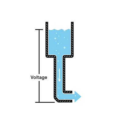![Water Tank Analogy](https://cdn.sparkfun.com/assets/e/8/8/4/8/5113d1c3ce395fc87d000000.png)\n\n*This is a water tank at a certain height above the ground. At the bottom of this tank there is a hose.*\n\n</div>\n\nThe pressure at the end of the hose can represent voltage. The water in the tank represents charge.\nThe more water in the tank, the higher the charge, the more pressure is measured at the end of the hose.\n\nWe can think of this tank as a battery, a place where we store a certain amount of energy and then release it.\nIf we drain our tank a certain amount, the pressure created at the end of the hose goes down.\nWe can think of this a as a decreasing voltage, like when a flashlight gets dimmer as the batteries run down.\nThere is also a decrease in the amount of water that will flow through the hose.\nLess pressure means less water (current) is flowing.\n\nBatteries are designed to provide a specific amount of voltage, and while bulbs itself don't have voltage, they require a specific voltage (electrical pressure) to work.\nRather, voltage is supplied to it from the electrical system for it to function, converting that electrical energy into light and heat.\nVoltage is the \"push\" that makes current flow through the bulb's filament or LED, causing it to light up.\n\n## Voltage Intuition\n\nI feel like even with these definitions of voltage as a potential difference, it is not very intuitive how exactly it works within circuits.\nAfter many many days of searching for answers I found some analogies that finally make sense and I wanted to share.\n\nIn a standard single-loop circuit (like a series of Christmas lights), voltage is \"spent\" as current flows through resistive components.\nIn the real world, even the copper wire acts as a resistor, though super weak.\nWhile we often pretend wires are perfect conductors in circuit diagrams (0 Ohms), physically, copper is not a super conductor.\nIt resists the flow of electrons slightly, which causes a slight loss of energy (voltage) as the current travels from one end to the other.\nCopper atoms vibrate, and in doing so collide with moving electrons. Every collision loses a bit of energy to heat or other forms. This loss of energy manifests a slight Voltage drop.\nIf you run electricity through a long distance wire, the resistance can add up over time, and reduce the voltage received on the other end.\n\nI want to use a ski slope as an analogy to explain how voltage works in a single-loop circuit.\nImagine the battery as a ski lift taking you to the top of the mountain (10V).\nEvery resistor or light bulb represents a slope, and as you ski down a slope, you lose height.\nAt the very top of the mountain, let's say you are at 10V. After the first resistor, you could be measured at 7V. After the second resistor, you might be at 3V.\nAnd at the bottom of the mountain, you are measured at 0V.\nIn this analogy, voltage represents the potential gravitational energy (height difference between you and the **ground**).\nThis concept of **GND** (ground) can also be commonly found within most circuit diagrams and it represents the point of lowest voltage in the entire circuit (0 V, end of the flow of current).\n\nWhen a wire splits into two or more branches, the voltage across each branch is the exact same.\nAll branches connect to the same split point, and reunion point, therefore the potential difference must be the identical.\nThink of it as a river flowing downhill. The stream hits an island and splits into 2 streams: Stream A is wide and clear, Stream B is narrow and rocky.\nThe river splits into 2 streams that both start at the same height and both streams merge again at the same height too.\nUsing this analogy, the drop in height (voltage) for both streams should be equal since they have the same starting and finishing elevation, even though one stream might carry much more water (current).\nNo matter how many slopes (resistors) a stream (parallel path) may encounter on the hill, it will drop the same height (voltage) as the other stream (other parallel path).\n\nUsing height to visualize voltage and gravity to visualize the pressure of voltage, made voltage extremely more intuitive for me.\n\n## Pulling Voltage (Visualizing Current)\n\nThis is a short one, but I wanted to briefly go over this because it is important to remember.\nNow, throughout this article voltage is described as the force that \"pushes\" electrons (or electrical charges) throughout the circuit.\nWhile this is actually an accurate definition for voltage, I don't like it very much because it makes visualizing voltage much more unintuitive.\nI would like to clarify a common misconception this creates when it comes to the flow of electrons.\nThis definition makes people commonly visualize the flow of electrons in a circuit as being pushed out of a power source, but that is actually not how it works.\nA better approach to visualize it is: to see the electrons being pulled by the ground from the power source (the other way around), like tug of war between the electrons.\nThis works well with the gravitational force analogy for voltage as well since gravity is a force that pulls (not pushes).\nThis is more intuitive when explaining why current doesn't flow in open circuits and explaining other mistakes where current is misinterpreted/misused.\n\nI'm guessing that is why current is conventionally shown flowing from the positive terminal to the negative terminal of a battery even though the flow of electrons is in the opposite direction.\nThat definitely makes it much easier to visualize electron flow.\nAlso conventionally, the positive terminal of a battery actually represents a high voltage and the negative terminal represents ground.\nThis might seem unintuitive at first because the positive terminal actually feels the least electrical pressure (voltage definition) to move electrons.\nWhen a point has a higher voltage than another point in a circuit, it basically means that it is more positive (has less electrical charge).\nThis works well with the pulling perspective of voltage, since a point of higher voltage has a stronger pull on electrons than a point of lower voltage.\n\nSo please keep this in mind throughout the article and whenever you think about current visually.\n\n## Ohm's Law\n\nTo further explain the relationship between voltage, current, and resistance:\n\n<div align=\"center\">\n\n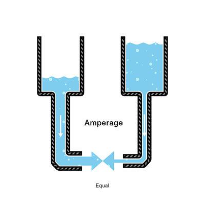![Ohm's Law Water Analogy](https://cdn.sparkfun.com/assets/7/6/4/b/6/5113dc8fce395fe201000001.png)\n\n</div>\n\nIf we increase the amount of water (charge) in the right tank, we increase the pressure (voltage) on the water (charge) from gravitational forces (electromagnetic forces).\nIn turn, even though the hose is narrower (more resistance) on the right side than the left, we still see an equal amount of water flowing (current) out of the right pipe.\nIf we increased the amount of water (charge) in the left tank, we increase the pressure (voltage), which increases the amount of water flowing (current) through the left pipe.\n\n- Water = Charge (measured in Coulombs)\n- Pressure = Voltage (measured in Volts)\n- Flow = Current (measured in Amperes, or \"Amps\" for short)\n- Hose Width = Resistance (measured in Ohms)\n\nAs explained by the analogy, Ohm combined the elements of voltage, current, and resistance to develop the formula of Ohm's Law: `V = IR`.\n`V` = Voltage in Volts, `I` = Current in Amps, and `R` = Resistance in Ohms.\n\n---\n\n# 2. Device Components\n\nBefore diving into circuits, it is helpful to understand the context of **device components** within **digital circuits**.\nWhile most physical variables in the real world (voltage, frequency, or position) are continuous (analog), digital systems abstract this information into discrete-valued variables.\nSpecifically, electronic computers generally use a binary representation, where a high enough voltage indicates a `1 (TRUE)` and a low enough voltage indicates a `0 (FALSE)`.\n\nThis digital abstraction allows designers to focus on the logical manipulation of 1s and 0s without constantly solving complex physics equations describing the motion of electrons in every component.\nDigital circuits are the physical implementations of this logic, restricting voltages to discrete ranges to represent binary states.\n\n## CMOS Transistors\n\nModern digital circuits are primarily built using **transistors**, which act as electronically controlled switches that turn ON and OFF when voltage or current is applied to a control terminal.\nThe two main types of transistors are *bipolar transistors* and *metal-oxide-semiconductor field effect transistors* (MOSFETs or MOS transistors, pronounced \"moss-fets\" or \"M-O-S\", respectively).\nThe specific technology used for the vast majority of chips today is known as CMOS (Complementary MOS).\nTo understand how these switches work, we must look at the underlying materials and components: semiconductors, diodes, and capacitors.\n\n### Semiconductors\n\n<div align=\"center\">\n\n![Conductivity Spectrum](https://i.imgur.com/Et6rtVd.png)\n\n</div>\n\nAn atom contains a nucleus of protons, surrounded by several orbital shells that contain a maximum amount of electrons.\nThe outermost orbital shell called the valence shell holds electrons with the most energy.\nThe electrons are held in place by the nucleus, however there's another shell called the conduction band.\nIf an electron can reach it, it can break free from the valence shell and move to another atom.\nWith a metal conductor like copper, the conduction band and valence shell overlap so it is very easy for the electron in the valence shell to move around freely.\nInsulators, have a valence shell which is packed and the conduction band is too far away to conduct electricity.\nIn **semiconductors**, there is one too many electrons in the valence shell (4 electrons) so they act as insulators.\nBut since the conduction band is close, if we provide some external energy, some electrons can gain enough energy to reach the conduction band and break free of the atom.\n\nBasically, a semiconductor materials ability to conduct electricity can be precisely controlled by adding impurities (doping) or applying voltage, light, or heat.\nThese semiconductor materials form the basis for transistors, diodes, and microchips that power modern electronics.\n\nCMOS technology relies on Silicon (Si), a group IV atom (so it has four electrons in its valence shell and forms bonds with four adjacent atoms) that forms a crystalline lattice.\nPure silicon turns out to be a poor conductor, so engineers add impurities called **dopants** to alter its conductivity.\nAdding Arsenic (group V) creates **n-type** silicon, which has free negatively charged electrons that act like negative charge carriers.\nAdding Boron (group III) creates **p-type** silicon, which has \"holes\" (missing electrons) that act like positive charge carriers.\n\n<div align=\"center\">\n\n![N-type and P-type Semiconductors](https://i.imgur.com/1qnjdDw.png)\n\n</div>\n\n### Diodes\n\nA **diode** is a semiconductor device, typically made of doped silicon, that essentially acts as a one-way switch for current.\nIt allows current to flow easily in one direction but severely restricts current from flowing in the opposite direction.\n\nI want to go on a slight tangent here real fast and explain the types of current as it is relevant to diodes and transistors.\nDC (Direct Current) flows steadily in one single direction (like from a battery), while AC (Alternating Current) periodically reverses direction, flowing back and forth in cycles (like wall outlets).\nAC is ideal for power grids because its voltage can be easily changed with transformers for efficient long-distance transmission, while DC is used by most electronics and batteries, often requiring conversion from AC.\nIf you were curious, power grids use generators and transformers that rotate magnets to precisely control voltage levels that push electrons back and forth.\n\"But how exactly?\" is beyond the scope of this study, and I will not be covering it here.\n\n<div align=\"center\">\n\n![DC vs AC Current Direction](https://i.imgur.com/fLfEv7w.png)\n\n</div>\n\nBack to topic. When n-type and p-type silicon are joined, they form a **diode**. A diode acts as a one-way valve for current.\nThe p-type region is called the anode and the n-type region is called the cathode.\nWhen the voltage on the anode rises above the voltage on the cathode, the diode is forward biased, and current flows through the diode from the anode to the cathode.\nBut when the anode voltage is lower than the voltage on the cathode, the diode is reverse biased, and no current flows.\n\nThe moment you join p-type and n-type material, nature tries to reach an equilibrium through a process called **diffusion**.\nDiffusion is simply the process of the high-concentration electrons from the n-type region rushing across the border to fill the \"empty holes\" in the p-type region.\nWhen an electron meets a hole at the junction, they cancel each other out and stick in place.\n\nOn the n-side, you have atoms like Phosphorus with 5 valence electrons. Since they only need 4 electrons to bond, that 5th electron is free to roam.\nHowever, the phosphorus atom is still electrically neutral because it has 15 protons and 15 electrons.\nOn the p-side, you have atoms like Boron with 3 valence electrons. They are also electrically neutral with 5 protons and 5 electrons, but they leave a \"hole\" in the lattice.\n\nWhen the junction is formed, those tightly packed free electrons from the n-side jump across to fill the holes in the p-side.\nAs a result, the Phosphorus atom on the n-side just lost an electron making it a positive ion and the Boron atom on the p-side just gained an electron making it a negative ion.\nBecause these atoms are locked into the solid crystal lattice, they cannot move.\nYou are left with a layer of stationary positive charge near the junction on the n-side and a layer of stationary negative charge near the junction on the p-side.\n\n<div align=\"center\">\n\n<img src=\"https://i.imgur.com/cWB9QSH.png\" alt=\"PN Junction Diagram\" width=600 />\n\n*PN junction showing the depletion region with stationary ions, free electrons, and holes.*\n\n</div>\n\nThis creates something called the **depletion region** at the PN junction, which contains no mobile charge carriers and only stationary charged ions.\nIn physics, whenever you have a separation of positive and negative charges that are fixed in space, an **electric field** is automatically created, and such is the case here.\nThese stationary ions near the junction create an internal electric field within the depletion region that acts like a wall, stopping any further electrons from crossing.\nThe internal electric field applies a force that repels negative charges from the n-side and repels positive charges from the p-side.\nI know, the diagram above looks SO misleading and it honestly is extremely unintuitive.\nThe negative and positive symbols within the depletion region represent the charge of the ions, and the other symbols in the n-side and p-side represent free electrons and holes. Two very different things.\nThe electric field suggests that positive charges experience a force that pushes them towards the negatively charged p-side and negative charges experience a push towards the positively charged n-side.\nThat is what the diagram actually means.\n\nBasically, this electric field creates a **potential barrier** which is simply the voltage equivalent of that field.\nFor electrons to cross the junction, a voltage bigger than the potential barrier needs to be applied.\nThink of it like: the electric field is the steepness of the slope, and the voltage is the height of the hill.\n\nYou might be wondering: \"why don't all the electrons just cross over until all holes are filled?\"\nReally, it's a balance of the two forces we talked about: diffusion and drift.\nThe natural tendency for electrons to cross over to fill the holes in the p-side (diffusion) and the repulsive force from the potential barrier (drift).\nThe depletion region stops growing the exact moment the electric field becomes strong enough to counteract the force of diffusion.\nThis state is known as equilibrium.\n\nBefore I dive into forward and reverse bias of a diode, I strongly recommend you to refresh your memory of the current intuition I explained earlier and really ingrain that pulling perspective of current.\nWhen you apply a **forward bias** to a diode, you connect the positive terminal (high voltage) to the p-side and the negative terminal (or ground) to the n-side.\nIn turn, electrons are pulled away from the p-side (pushed into n-side), breaking the equilibrium, overcoming the voltage produced by the potential barrier, squashing the depletion region and allowing current to flow through.\nHowever, when you apply a **reverse bias**, you connect the positive terminal (high voltage) to the n-side and the negative terminal (or ground) to the p-side.\nThis results in electrons being pulled away from the n-side junction, and in consequence pushes holes away from the p-side junction (widening the depletion region).\nSince the free electrons (negative charge carriers) are pulled away from the junction, and empty holes (positive charge carriers) are pushed away from the junction, we are left with a wider depletion region at the junction of the diode filled with ions which strengthen the electric field and potential barrier even more.\nSo, a reverse biased diode acts as a strong insulator with very microscopic leakage of current.\n\nQuick tangent to make sure you understand!\nIn forward biased diodes, we can say \"electrons are pulled from the p-side and pushed into the n-side of the diodes\" because current flows through diodes in forward bias.\nHowever, it is not the case for reverse biased diodes. In reverse biased diodes, electrons feel a pulling force from the n-side which attract the electrons away from the junction.\nThis causes holes to be pushed away from the junction as well which causes the widening of the depletion region, blocking current.\nHowever, there are no electrons being pushed into the p-side of the diode because the electron tug of war ends at the PN junction of the diode.\nRevisit my notes on visualizing current (find in table of contents) if you don't understand what I am trying to get at here.\n\nAll of that combined together should intuitively explain the exact science behind how diodes act as one-way valves for current.\nHere is a quick [video](https://youtu.be/Fwj_d3uO5g8) to help visualize and understand the physics behind a diode.\n\nQuick note! Diodes don't always allow current to flow in forward bias though.\nA silicon diode requires a specific minimum voltage (known as the forward voltage drop ~ 0.6-1.0 V) to overcome its potential barrier before conducting electricity, after which current increases exponentially.\nEven though diodes block current with reverse bias, if the reverse voltage is high enough (exceeding the diode's reverse breakdown voltage), it will conduct, but this usually causes permanent failure.\n\n<div align=\"center\">\n\n![Diode Symbol and Operation](https://i.imgur.com/RjCRjuf.png)\n\n*The diode symbol intuitively shows that current only flows in one direction.*\n\n</div>\n\n### Capacitors\n\nA **capacitor** is an electrical circuit component that temporarily lets current flow through and temporarily stores electrical energy (like a battery).\nIt contains two conductive plates separated by an insulating dielectric.\nA dielectric is an electrical insulator (glass, ceramic, plastic, etc) that supports an electrical field by becoming polarized, meaning its charges shift slightly but doesn't allow for current to flow.\nThis layer is essential, as it allows a voltage to develop across the plates by holding an electric charge instead of letting current flow between them.\n\nIn simple terms, the capacitance of a capacitor is the measure of capacitor's ability to store electrical charge onto its plates.\nThe ratio of stored charge `Q` to the applied voltage `V` gives the capacitance `C`: `C = Q / V`.\nIt is slightly unintuitive at first, but once you realize that charge and voltage are completely separate, capacitance starts to make more sense.\nThink of it like: a bucket's size (Capacitance) is independent of how much water (Charge) is in it or how much pressure (Voltage) is at the bottom.\nWhen a voltage `V` is applied to one of the conductors, the conductor accumulates electric charge `Q` and the other conductor accumulates the opposite charge `-Q`.\nWhile we often describe the charge as being held on the plates, the energy is more accurately stored in the electric field between them.\nAs current flows into the capacitor, the field strengthens, and as it discharges, the field weakens, releasing the stored energy back into the circuit.\n\nCapacitance, measured in Farads (F), depends on several factors: the area of the conductive plates, the thickness and type of dielectric material, and the separation distance between the plates.\nA larger plate area or smaller distance gap between them increases capacitance, allowing the capacitor to store more charge at a given voltage.\nTo show how these variables are related, you can also measure the capacitance of a capacitor using this formula: `C = \ud835\udf00 * (A / d)`.\n`\ud835\udf00` represents the permittivity (ability to store electrical energy in an electric field) of the dielectric material, `A` represents the area of the conductive plate, and `d` represents the distance between them.\n1 Farad means the capacitor can hold 1 Coulomb of charge across a potential difference of 1 Volt.\nYou will more commonly see capacitors measured in pico-farads (pF), nano-farads (nF) or micro-farads (\u03bcF).\n\nWhen a voltage is applied and electrons gather on a plate, the dielectric becomes positively charged near the negatively charged plate and vice versa. This process is called polarization.\nThe dielectric is influenced by the surrounding conductive plates to have a shift in its electron cloud which creates a tiny internal electric field.\nThe two oppositely charged conductive plates separated by the dielectric also begin to form a larger external electric field.\nThe dielectric not only helps as an insulator between the plates but also uses its internal field to oppose the external field of the plates.\nIt's important to note that this is an intended feature of the dielectric because it helps slow the growth of the opposing voltage from the external field, which in turn increases the capacitance of the capacitor.\nThe external electric field is strong enough to hold the charges in these plates until connected to another circuit to discharge the capacitor.\n\n<div align=\"center\">\n\n![Capacitor Circuit Diagram](https://i.imgur.com/QF97Qta.png)\n\n</div>\n\nBefore I begin explaining how charging and discharging a capacitor works, I want to explain how circuits actually work with capacitors since they are physically open circuits.\nBoth conductive plates within the capacitor have a bunch of electrons randomly roaming around much like the copper wire of any circuit.\nInitially, when the capacitor is fully discharged, the plates are both electrically neutral and no energy or charge is stored yet.\nOnce you start charging the capacitor, electrons start to build up on one of the plates, drawing positive charge from the dielectric toward it and pushing the negative charge within the dielectric away.\nThis forms an electrical field around the capacitor which begins to push the electrons of the other plate out.\nThis creates the illusion of current \"flowing through\" the capacitor even though there are no electrons passing through the capacitor because of the insulator between the plates.\nIt is important to note that positive charges (protons) don't move since all the atoms are tethered in the solid dielectric, it is just the shifting electron clouds that create dipoles in the dielectric.\n\n<div align=\"center\">\n\n![RC Circuit](https://i.imgur.com/LIfrOXz.png)\n\n*RC circuit: a capacitor (C) in series with a resistor (R), connected to a battery (V_s) through a switch.*\n\n</div>\n\nThe circuit above contains a capacitor (`C`) in series with a resistor (`R`), both connected to a battery power supply (`V_s`) through a mechanical switch.\nAt the instant the switch is closed, the capacitor starts charging up through the resistor.\nThis charging process continues until the capacitor's voltage is equal to the battery supply's voltage.\n\n<div align=\"center\">\n\n![Capacitor Voltage vs Time](https://i.imgur.com/MUxUUPf.png)\n\n*Capacitor voltage (V_c) approaching supply voltage (V_s) over time during charging.*\n\n</div>\n\nAs the capacitor starts charging, charge builds up on its plates, creating an increasing voltage `V_c` that opposes the battery voltage `V_s`.\nThis opposition reduces the current slowly as the voltage `V_c` approaches `V_s`, resulting in exponential decrease in current over time.\n\nThis charging behavior follows a time constant represented by: `\ud835\udf0f = RC`.\n`R` represents the resistance of the circuit in Ohms, and `C` represents the capacitance of the circuit in Farads.\nThe time constant `\ud835\udf0f` represents the time required for the capacitor to reach ~63% of its full charge potential.\nThe value of `\ud835\udf0f` depends on the resistance `R` and capacitance `C`: a larger `R` slows the charging rate, while a larger `C` allows the capacitor to hold more charge, also requiring more time to reach full charge.\n\nAs time progresses, the voltage across the capacitor follows an exponential curve, increasing quickly at first but slowly as it approaches `V_s`.\nAt around `5\ud835\udf0f`, the capacitor voltage `V_c` has essentially reached `V_s`, and we consider it fully charged.\nAt this point, known as the Steady State Period, the capacitor behaves like an open circuit, holding the fully supply of voltage across it, while current falls to 0, and the total charge reaches `Q = CV`.\nThe stored charge will forever stay in the capacitor and won't be lost until connected to another circuit. However, capacitors do leak charge in practice.\nNote that theoretically, the capacitor never actually reaches 100% of its full charging potential.\nEven after `5\ud835\udf0f`, the capacitor only reaches 99.3%, but for all practical purposes, we can consider that capacitor fully charged at this point, as there is hardly any change after this.\n\n<div align=\"center\">\n\n![Capacitor Discharging Example](https://i.imgur.com/8VtYd7e.png)\n\n*A capacitor and bulb in parallel \u2014 when the switch opens, the capacitor discharges to keep the bulb lit.*\n\n</div>\n\nNow, take the circuit above with a capacitor and a bulb connected in parallel powered by a battery power supply through a mechanical switch.\nWhen we close the switch, current flows through the circuit and charges up the capacitor and lights the bulb in parallel.\nIf we let the capacitor charge for a while and then open the switch, you can see that the bulb actually stays lit since the capacitor immediately starts discharging and releases its charge back into the circuit.\nThe bulb will stay lit until the capacitor is done discharging, meaning it is back to its default state and the plates have an equal charge again.\nIf we mimic a pulsating DC by repeatedly flipping the mechanical switch of the circuit, the bulb will stay lit all the time because it is being powered by the battery when the switch is closed and being powered by the capacitor when the switch is open.\nThis demonstrates how a capacitor can smoothen out the ripples that can appear while converting AC to DC.\n\nAdditionally, while a capacitor is placed in a DC circuit, it charges up to match the supply voltage, and once charged, it effectively blocks the flow of current.\nIn an AC circuit however, the capacitor behaves differently.\nSince AC consistently changes direction, the capacitor repeatedly charges and discharges, creating an effect that lets AC current \"pass through\" the capacitor.\n\nHere is a quick [video](https://youtu.be/X4EUwTwZ110) that visually explains how electricity \"flows through\" the capacitor.\n\n### Current Rectification\n\nOur homes are powered by power grids that provide an AC to our wall outlets.\nAnd our electronic devices need to convert the AC from these outlets to DC because most sensitive electronics (computers, phones, etc.) run on a steady, one-way flow of electrons (DC), not the fluctuating AC waveform.\nOur devices convert AC to DC using a process called **rectification** typically involving: a transformer to adjust the voltage, a rectifier circuit (diodes) to change AC to pulsating DC, a capacitor to smooth the ripples, and a voltage regulator to provide a steady, constant output for electronics.\n\n<div align=\"center\">\n\n<img src=\"https://i.imgur.com/GJHft6R.png\" alt=\"Full-Wave Rectifier Circuit\" width=\"400\" />\n\n*Diagram of a circuit that shows how a full-wave rectifier is constructed.*\n\n</div>\n\nThis is a breakdown of all the steps in the rectification process:\n\n1. **Step-Down Transformer**: The high AC voltage from the wall outlet is reduced to a lower, more manageable AC voltage level for the device.\n2. **Rectifier (Diodes)**: Diodes allow current to flow in only one direction.\n    - **Half-wave rectification**: Blocks the negative half of the AC wave, resulting in a pulsating DC.\n    - **Full-wave rectification**: Uses four diodes to flip the negative half of the wave, making it positive, creating a smoother, but still bumpy, DC output. Check the figure above to visualize the circuit.\n3. **Filter (Capacitor)**: A capacitor charges up during the peaks of the pulsating DC and discharges during the dips, smoothing out the ripples and creating a steadier DC.\n4. **Voltage Regulator**: The regulator ensures a precise, constant DC voltage by compensating for any remaining fluctuations, providing the stable power needed for sensitive electronics.\n\n## nMOS vs pMOS\n\nMOSFETs are kind of like sandwiches that consist of layers of conductive and insulating materials. These MOSFETs are built on thin and flat **wafers** like most modern electronics.\nA wafer is a thin slice of semiconductor material, typically high-purity crystalline silicon, used as the substrate for fabricating integrating circuits (chips) in electronics.\nThese thin, usually circular discs (15 - 30 cm in diameter) serve as the foundational base upon which microelectronic devices are manufactured through processes like doping, etching, and deposition.\n\nThe manufacturing process of a MOSFET obviously begins with a bare wafer, and then involves a sequence of steps in which dopants are implanted into the silicon, thin films of silicon dioxide and silicon are grown, and metal is deposited.\nBetween each step, the wafer is carefully and precisely patterned by very accurate and advanced laser technology so that the materials appear exactly where they are desired.\nSince transistors are literally a fraction of a micron (1e-6 m) in length, an entire wafer is processed at once.\nOnce the processing is complete, the wafer is cut into tiny rectangles called **chips** containing millions or billions of transistors.\nThese chips are first tested, and then placed in a plastic or ceramic package with metal pins on the bottom to connect them to circuit boards.\n\n<div align=\"center\">\n\n<img src=\"https://i.imgur.com/mTtlJpJ.png\" alt=\"Silicon Wafer\" width=\"400\" />\n\n*An example of a silicon wafer body and the chips that it gets broken into.*\n\n</div>\n\nSpecifically, MOSFET sandwiches consist of 3 main layers: a conductive layer on the top called the gate, an insulating dielectric layer of silicon dioxide (`SiO_2`) in the middle, and the silicon wafer called the substrate on the bottom.\nIf you were wondering, silicon dioxide is basically just glass and also often simply called *oxide* in the semiconductor industry.\nHistorically, the gate was constructed from metal, hence the name metal-oxide-semiconductor, however, modern manufacturing processes use polycrystalline silicon for the gate because it doesn't melt during some of the following high-temperature processing steps.\nThe gate acts as the switch that stops and allows current to flow through the MOSFET when there is a voltage applied across the source and drain.\n\n<div align=\"center\">\n\n![nMOS and pMOS Cross Sections](https://i.imgur.com/5bn2gNE.png)\n\n*Cross-sectional view of nMOS (left) and pMOS (right) transistors showing the source, gate, and drain terminals.*\n\n</div>\n\nAs shown by the figure above, there are two flavors of MOSFETs: nMOS and pMOS. The figure illustrates the cross section of the nMOS and pMOS from the side.\nThe n-type transistors, also known as nMOS, have 2 separate regions of n-type dopants neighbouring the gate (called the **source** and **drain**) that were planted onto a p-type semiconductor substrate base.\nThe pMOS transistors are just the opposite, consisting of a p-type source and drain regions in an n-type substrate base.\n\nNow you're probably wondering: \"why are there 2 flavors of MOSFETs and what's the difference between how they function?\"\nBefore I get into that, I want to first dive into the nMOS transistor and how the components we learned about earlier come together to operate this transistor.\nAfter that, I can explain how pMOS constructions and operations contrast from nMOS.\n\n### Working principle of nMOS\n\nThe source and drain of a MOSFET are both connected to regions of n-type dopants that are embedded into the top of the p-type wafer substrate like shown in the diagram.\nDoesn't this look familiar? The n-type regions that were embedded into the p-type substrate actually create two back to back **diodes** within the MOSFET from source to body and drain to body.\nThe PN junction between these regions and the substrate actually form a depletion region which blocks electrons from crossing when there is no voltage applied across the source and diode.\n\n> **When the gate (the switch of the MOSFET) is OFF but there is a voltage applied across the source and drain of an nMOS, what is stopping current from flowing through?**\n\n> Before I begin explaining, it might be helpful to revisit how diodes work and understand the pulling voltage intuition better.\n> So when the gate is electrically neutral, meaning there has been no voltage applied to it yet, but there is a voltage across the source and drain, MOSFETs block current from flowing through as designed to.\n> The question is not why, but how? Think of how the electrons are moving. The voltage applied pulls the electrons from the ground which the drain is attached to.\n> Basically, electrons within the drain experience a pulling force from the ground which pull electrons away from the PN junction making the depletion region wider.\n> In simple terms, the current is trying to flow through a reverse biased diode which we have learned acts as an insulator, therefore blocking the current from \"leaking\" from the drain into the floor of the chip.\n> This is a brief explanation as to how reverse biased diodes block current, read the notes on diodes for more in depth explanations.\n> Ultimately, for a diode to pass current, it needs to be forward biased (p-type region has a higher voltage), but in the case of an nMOS transistor the p-type substrate is connected to Ground (0V).\n> No matter how much voltage is provided to the drain, the diodes will forever be reverse biased.\n\nIf you haven't noticed already, the metal-oxide-semiconductor sandwich we manufactured earlier actually forms a **capacitor**. Take a look at the figure of an nMOS transistor above.\nThere is a thin insulating dielectric layer (from the silicon dioxide) that separates the two conductive plates which are the polysilicon gate on top and the silicon wafer substrate on the bottom.\nA MOSFET behaves as a voltage-controlled switch in which the gate voltage with the support of the dielectric creates an electric field that turns ON or OFF a connection between the source and drain, hence the name **field effect transistor**.\n\n<div align=\"center\">\n\n![Field Effect Transistor Diagram](https://i.imgur.com/qhU9mNq.png)\n\n*Visualization of the electric field and inversion layer forming under the gate of an nMOS transistor.*\n\n</div>\n\n> **How does an nMOS allow current flow through the source and drain when the gate is ON?**\n\n> By applying a positive voltage to the gate, the power source (like a battery) is effectively sucking electrons out of the gate material, making the gate positively charged.\n> Since the gate is now positively charged and the dielectric is an insulator, those \"missing\" electrons can't be replaced by the substrate below, instead creating a static electric field.\n> The electric field becomes strong enough for the positively charged gate to act like a magnet for negative charges, pulling the free electrons in the p-type substrate towards the gate, and pushing the holes away.S\n> Since the electric field pulled the free electrons in the p-type substrate, it temporarily disables the depletion layers at the PN junctions.\n> As those electrons pile up against the bottom of the dielectric, they form a thin but highly concentrated layer of negative charge called the **inversion layer**.\n> Since this layer is full of electrons, this specific part of the p-type substrate behaves like n-type silicon and creates a channel (or bridge) for electrons to flow from the source to the drain.\n> Refer to the visual above or watch the [video](https://youtu.be/IcrBqCFLHIY) (where I grabbed it from) to visualize it better.\n\n<div align=\"center\">\n\n![nMOS Operation States](https://i.imgur.com/siTVtdw.png)\n\n*nMOS transistor in OFF state (left) and ON state (right) showing channel formation.*\n\n</div>\n\n> **If the MOSFET uses the physical structure of a capacitor, the gate stores the charge accumulated when a voltage is applied, so how do you turn the nMOS OFF?**\n\n> Because the gate oxide is such a high quality insulator, if you apply +5V to the gate and then simply cut the wire (leaving the gate floating), the charge has nowhere to go.\n> The nMOS would stay ON indefinitely or until the all the charge slowly leaks out.\n> To actually turn the transistor OFF, you can't just stop applying the positive voltage to the gate, you have to actively drain the charge.\n> In most digital circuits (like the processor in our computers), the gate is connected to a \"driver\" circuit.\n> To turn the nMOS ON, the driver connects the gate to the Supply Voltage (`V_dd`). To turn the nMOS OFF, the driver flips a switch and connects the gate to Ground (V_ss).\n> By connecting the gate to Ground (an ocean of electrons), you provide a low-resistance path for those stored electrons to rush back into the gate, neutralize the positive charge and kill the electric field.\n> Looking into how the driver circuit works is not within the scope of the study but still encouraged if you are interested!\n\n<div align=\"center\">\n\n<img src=\"https://i.imgur.com/HWZnJf8.png\" alt=\"BJT vs MOSFET Comparison\" width=600 />\n\n*Comparison of BJT (current-controlled) and MOSFET (voltage-controlled) transistor operation.*\n\n</div>\n\n> **Why do transistors today use a capacitor structure?**\n\n> Using a capacitor (for the \"Field Effect\") instead of a direct connection (like the \"Current Effect\") in older Bipolar Junction Transistors (BJT) was one of the most important design choices in human history.\n> In older BJT transistors, you have keep pushing current into the base to keep it on which constantly wastes energy.\n> In a MOSFET, however, once you charge the capacitor, no more current flows, and it stays ON for free.\n> That's the main reason why your phone doesn't get hot just sitting in your pocket even with the screen off. I'm not interested in diving deep into BJTs here since it is outdated technology.\n> Also, since the gate is completely insulated by the capacitor's dielectric, we can control larger electric components like massive motors with a tiny microprocessor and not have to worry about any high power leaking back into the processor which could potentially fry it.\n> Capacitative gates are also much easier to shrink, and as you make a MOSFET smaller, you make the \"capacitor\" smaller, making it faster to charge and discharge.\n> This allowed engineers go from fitting a few thousand transistors in a chip to billions today, keeping Moore's Law alive.\n> Watch this [video](https://youtu.be/MiUHjLxm3V0) by Veritasium about modern transistors to understand the latest advancements in transistor technology.\n\n### Working principle of pMOS\n\nMatter of fact, the operations of a pMOS transistor are the exact opposite than that of an nMOS transistor.\nThe only difference between the construction of a pMOS and nMOS is the wafer substrate and the dopant regions.\nIn a pMOS transistor, the wafer body is actually doped as n-type silicon and the source and drain are both connected to regions of the wafer embedded with p-type dopants.\n\n<div align=\"center\">\n\n![CMOS Cross-Section Example](https://i.imgur.com/8Ng8qpR.png)\n\n*Cross-section showing how nMOS and pMOS transistors coexist on a single p-type wafer using n-wells.*\n\n</div>\n\nThat might make you curious, how do CMOS circuits combine nMOS and pMOS transistors to work together if their entire wafer bodies need to be doped differently?\nThis is where the magic of combining nMOS and pMOS together to give us CMOS technology comes into play.\nWe actually start with a single p-type wafer (connected to Ground), and then \"dig\" little swimming pools of n-type silicon dopants into it called **n-wells**.\npMOS transistors sit within these n-wells as they require an n-type body to operate with more p-type dopants implanted into the n-wells.\n\nLogically, the pMOS functions as the exact opposite from the nMOS transistors, but that is a mere illusion as they actually operate very similarly.\nThe nMOS is OFF when the gate experiences no voltage and ON when a positive voltage is applied to the gate.\nThe pMOS works the opposite way, meaning it is ON when the gate experiences no voltage, but OFF when the gate experience a positive enough voltage.\nHowever, the pMOS doesn't exactly work the way you might initially imagine.\n\nIn the vast majority of CMOS circuits, the source and wafer body are tied to the same wire.\nIn an nMOS, the source and body are both connected to ground because it is the Source's job to provide electrons and the Body's job to reversely bias the diodes with what the source provides and the drain demands.\nConnecting the p-type wafer of an nMOS to ground pushes electrons into the wafer, neutralizing the electric field between the gate and the body, and keeping the diodes reverse biased by holding the depletion regions strong.\nSimilarly, in a pMOS, the source and body are both connected to the point of highest voltage (`V_DD` ~ +5V).\nIn the case of pMOS, it is the Source's job to provide holes to the circuit and the Body's job to provide a high enough voltage to the n-type substrate such that the p-type source and drain can never have a higher voltage, keeping them reverse biased.\nSo the source-body and drain-body diodes will be forever reverse biased by default because the Body is tied to the highest voltage in the circuit.\n\n<div align=\"center\">\n\n<img src=\"https://i.imgur.com/LLJHNQI.png\" alt=\"CMOS Logic Gate Structure\" />\n\n*CMOS logic structure showing the Pull-Up Network (pMOS) and Pull-Down Network (nMOS).*\n\n</div>\n\nHowever, since the substrate is tied to a high positive voltage, when the gate is electrically neutral (0V), an electric field across the dielectric is formed.\nThis electric field points in the opposite direction than that of an nMOS and repels the free electrons in the n-type substrate but attracts the holes from the source, drain, and body.\nThis creates a thin inversion layer at the bottom of the dielectric of p-type silicon in the n-type substrate and temporarily disables the depletion layer at the PN junctions.\nThe channel formed also allows holes (positive charge carriers) to flow from the source to the drain.\nIn reality, electrons are jumping from the drain, into the holes of the body, and moving towards the source and current is flowing in the opposite direction.\nConventional current in nMOS transistors flows from drain to source, but source to drain in pMOS transistors.\n\nWhen you provide a positive voltage to the gate that is equal to the source/body, the electric field across the dielectric gets neutralized, and the diodes are back to being reverse biased to block current.\nEven though pMOS is constructed differently, the way the pMOS operates is the exact same as the nMOS.\nHowever the operation of a pMOS creates the \"logical illusion\" of being completely opposite to that of an nMOS transistor.\nUltimately, when the gate is connected to Ground (0V) the pMOS is considered ON, and when the gate is connected to (`V_DD` ~ +5V) it is considered OFF, making the pMOS the logical opposite of the nMOS transistor.\n\n### Why both flavors?\n\nUnfortunately, MOSFETs are not perfect switches. CMOS circuits face a physical limitation called the Threshold Voltage (`V_th`).\nTo understand this, you have to remember that a MOSFET follow the source voltage when it's trying to pass a signal.\nIn an nMOS, the gate needs to have a slightly higher voltage than the voltage it is trying to move, and in pMOS, the gate needs to have a slightly lower voltage than the voltage it's trying to move.\nnMOS is very good at passing 0s because whether the gate is \"closed\" or \"wide open\", it passes a strong 0 since the source voltage is already 0.\nWhen trying to pass a +5V signal, the source voltage slowly starts to increase but eventually stops around 4.3V (for a 0.7 threshold voltage) to keep the transistor ON.\nTherefore nMOS transistors are weak when trying to pass 1s.\nOn the contrary, pMOS is good at passing 1s for the exact same reason.\nWhen trying to pass a 0V signal, the source voltage slowly starts to decrease but eventually stops around 0.7 V (because of the threshold) to keep the transistor OFF.\n\nSince nMOS is bad at passing 1s and pMOS is bad at passing 0s, CMOS technology uses them in complementary pairs majority of the time (hence the name \"Complementary MOS\").\nIn digital logic, specifically CMOS, every logic gate is divided into two separate halves that works together: the **Pull-Up Network (PUN)** and the **Pull-Down Network (PDN)**.\nTheir job is to ensure the output pin is always connected to either High (`V_DD`) or Low (`GND`), and never both at the same time.\nI will dive deeper into driver circuits, gate networks, and more in the next study talking about circuits and logic. Stay tuned!\n\n---\n\n# Resources\n\n- [csl.cornell.edu/courses/ece2300](https://www.csl.cornell.edu/courses/ece2300/readings.html)\n- \"Digital Design and Computer Architecture, RISC-V Edition,\" by D. M. Harris and S. L. Harris (Morgan Kaufmann, 2021)\n- [Making logic gates from transistors - YouTube](https://youtu.be/sTu3LwpF6XI)\n- [learn.sparkfun.com (physics of electricity)](https://learn.sparkfun.com/tutorials/voltage-current-resistance-and-ohms-law/all)\n- [fluke.com/blog/electrical/diode (what is a diode)](https://www.fluke.com/en-us/learn/blog/electrical/what-is-a-diode)\n- [florisera.com/capacitors (what is a capacitor)](https://florisera.com/introduction-to-capacitors/)\n\n---\n\n*Written by BooleanCube :]*\n",
      "toc": [
        {
          "level": 1,
          "id": "1-physics-behind-electricity",
          "title": "1. Physics Behind Electricity"
        },
        {
          "level": 2,
          "id": "voltage-intuition",
          "title": "Voltage Intuition"
        },
        {
          "level": 2,
          "id": "pulling-voltage-visualizing-current",
          "title": "Pulling Voltage (Visualizing Current)"
        },
        {
          "level": 2,
          "id": "ohms-law",
          "title": "Ohm's Law"
        },
        {
          "level": 1,
          "id": "2-device-components",
          "title": "2. Device Components"
        },
        {
          "level": 2,
          "id": "cmos-transistors",
          "title": "CMOS Transistors"
        },
        {
          "level": 3,
          "id": "semiconductors",
          "title": "Semiconductors"
        },
        {
          "level": 3,
          "id": "diodes",
          "title": "Diodes"
        },
        {
          "level": 3,
          "id": "capacitors",
          "title": "Capacitors"
        },
        {
          "level": 3,
          "id": "current-rectification",
          "title": "Current Rectification"
        },
        {
          "level": 2,
          "id": "nmos-vs-pmos",
          "title": "nMOS vs pMOS"
        },
        {
          "level": 3,
          "id": "working-principle-of-nmos",
          "title": "Working principle of nMOS"
        },
        {
          "level": 3,
          "id": "working-principle-of-pmos",
          "title": "Working principle of pMOS"
        },
        {
          "level": 3,
          "id": "why-both-flavors",
          "title": "Why both flavors?"
        },
        {
          "level": 1,
          "id": "resources",
          "title": "Resources"
        }
      ]
    },
    {
      "title": "Cracking The Technical Interview",
      "summary": "Learn my step by step outline of a perfect technical interview.",
      "tags": [
        "technical",
        "guide",
        "programming"
      ],
      "date": 1762178202000,
      "cover": "https://i.imgur.com/ABSMW3G.png",
      "hidden": false,
      "slug": "technical-interviews",
      "content": "After solving over 1,000 LeetCode problems, competing in ICPC for UCF, and successfully navigating technical interviews at companies like Google and Voloridge Investment Management, I've learned that technical interviews aren't just about knowing algorithms\u2014they're about having a systematic approach. In this post, I want to share the exact formula that's helped me succeed in some of the most challenging technical interviews in the industry.\n\n# Why Listen to Me?\n\nBefore diving in, let me establish some context. I've been on both sides of the technical interview process: as a candidate who's passed difficult interviews with flying colors at top tech companies and quantitative finance firms, and as someone who's spent thousands of hours honing problem-solving skills through competitive programming. My Google interview experience, in particular, crystallized a framework that I've since refined and used successfully in other high-stakes interviews, including my return offer for a Quantitative Developer position at Voloridge.\n\nThe patterns I'm about to share aren't theoretical\u2014they're battle-tested strategies that have worked consistently across different companies and interview styles.\n\n# The Landscape: Types of Technical Interviews\n\nNot all technical interviews are created equal. In my experience, they generally fall into three categories:\n\n**1. Coding Technical Interviews**  \nThese are your classic algorithm and data structure problems. You'll write code, optimize solutions, and demonstrate your problem-solving process. This is what most people think of when they hear \"technical interview.\"\n\n**2. Conversational Technical Interviews**  \nThese focus on system design, architecture decisions, or discussing your past projects in depth. You're explaining trade-offs, demonstrating technical judgment, and showing how you think about complex problems at a higher level.\n\n**3. Non-Coding Technical Interviews**  \nThese might involve whiteboarding without implementation, discussing theoretical concepts, or domain-specific knowledge assessments (especially common in quant roles).\n\nHere's the thing: for conversational and non-coding interviews, you need to be broadly prepared for anything. You need deep knowledge of your domain, experience to draw from, and the ability to articulate complex ideas clearly. There's no shortcut.\n\n**But for coding technical interviews? There's a formula.** And that's what this post is about.\n\n# The Formula: My Play-by-Play Approach\n\nThis framework comes directly from my Google interview experience, but I've used it successfully across multiple companies. It's not just about solving the problem\u2014it's about demonstrating your thought process, communication skills, and engineering maturity.\n\n## Step 1: Meet and Greet Your Interviewer\n\nThis might seem obvious, but those first 30 seconds matter. Be warm, be genuine, and remember that your interviewer is a human being who probably wants you to succeed and might be just as stressed as you. They're about to spend 45-60 minutes with you, so establish a positive rapport.\n\nI usually keep it simple: introduce myself, maybe make a brief comment about being excited for the interview, and then relate to them in some way. Don't overthink this part, but don't skip it either. For example, if they ask you \"how are you doing?\", don't just respond with \"I'm good, thanks.\" Try to relate to them by bringing up a story like: \"I'm doing great, I just came back from a refreshing walk and the weather was beautiful. What about you?\" This loosens up the tension on both sides and reminds the interviewer that you are also just a human and makes them feel like you are easy to work with.\n\n## Step 2: Listen and Read the Question Carefully\n\nWhen the problem appears on your screen or your interviewer starts explaining it, your job is simple: **listen actively** and **read every word**.\n\nI've seen candidates (and admittedly, I've done this myself in earlier interviews) who start thinking about solutions before fully understanding the problem. Resist this urge. If there's a written problem statement, read it twice. If it's verbal, consider taking notes.\n\n## Step 3: Clarify the Question IN DETAIL\n\nThis is where most candidates either make or break their interview. The difference between a good candidate and a great candidate often comes down to how thoroughly they clarify the problem before writing a single line of code.\n\nAsk questions like:\n\n- What are the constraints on the input size?\n- Can the input be empty? Can it contain negative numbers? Duplicates?\n- What should I return if there's no valid solution?\n- Are there any performance requirements I should be aware of?\n- Can I modify the input, or do I need to treat it as immutable?\n\nDon't be afraid to seem \"too thorough\" here. Interviewers want to see that you think about edge cases and constraints. I usually spend 2-3 minutes on this phase, and it's time well spent.\n\n## Step 4: Verbalize and Check Your Assumptions\n\nAfter asking clarifying questions, explicitly state your assumptions. This serves two purposes: it ensures you and your interviewer are on the same page, and it demonstrates that you think carefully about problem constraints.\n\nFor example: \"So just to confirm, I'm assuming the array is unsorted, all integers are positive, and we need to return the actual elements, not just their indices. Is that correct?\"\n\nWait for confirmation. If you're wrong, better to find out now than after you've coded a solution to the wrong problem.\n\n## Step 5: Explain Your First Solution (Brute Force/Naive Approach)\n\nHere's a crucial insight: **always start with the brute force solution, even if you immediately see the optimal approach.**\n\nWhy? Because it demonstrates several things:\n\n- You can identify a working solution quickly\n- You understand the problem well enough to solve it\n- You're methodical in your approach\n- You're not going to freeze if the optimal solution doesn't come to you immediately\n\nUse the whiteboard (or collaborative coding doc) to sketch out your approach. Explain the algorithm in plain English or pseudocode. Walk through an example.\n\n\"The first solution that comes to mind is a brute force approach where I check every possible pair. This would look like two nested loops...\"\n\n## Step 6: Ask If They Want You to Code It\n\nThis is a small but important step that many candidates skip. After explaining your brute force approach, explicitly ask:\n\n\"Would you like me to code this brute force solution first, or should I think about optimizing it?\"\n\nDifferent interviewers have different preferences. Some want to see you code something working before optimizing. Others would rather you skip straight to the optimal solution. By asking, you:\n\n- Show respect for their time and preferences\n- Avoid wasting time coding something they don't care about\n- Demonstrate that you're collaborative and communicative\n\n## Step 7: Think About Optimal Solutions\n\nIf they want you to optimize (or if your brute force isn't good enough), this is where you apply your algorithmic knowledge.\n\nThink out loud. Verbalize your thought process:\n\n- \"The bottleneck in the brute force is the repeated lookups... could I use a hash map to trade space for time?\"\n- \"I'm doing redundant work in these overlapping subproblems... this looks like a dynamic programming scenario.\"\n- \"If I sort the array first, I could use two pointers...\"\n\nDraw on your knowledge of common patterns: sliding windows, two pointers, hash maps, heaps, graphs, dynamic programming, etc. If you're stuck, talk through what you're thinking. Good interviewers will give you hints if they see you're on the right track.\n\n## Step 8: Explain Your Optimal Solution WITH WHITEBOARD\n\nOnce you've identified your optimal approach, don't just start coding. Take the time to fully explain it first, using the whiteboard or drawing tools.\n\nWalk through:\n\n- The high-level algorithm\n- The data structures you'll use\n- The time and space complexity\n- A concrete example with actual values\n\nThis serves as both a sanity check for you and a communication exercise. If there's a flaw in your logic, it's much easier to catch it here than after you've written 50 lines of code.\n\n## Step 9: Code the Optimal Solution\n\nFinally, it's time to code. By this point, you should have a clear roadmap of what you're building.\n\nAs you code:\n\n- Talk through what you're doing (\"I'm initializing a hash map to store...\")\n- Write clean, readable code with meaningful variable names\n- Think about edge cases as you go\n- Test your code mentally or with a simple example\n\nIf you realize you made a mistake, don't panic. Explain what you noticed and how you're going to fix it. Interviewers care more about your debugging process than whether you got it perfect on the first try.\n\n# Why This Formula Works?\n\nThis systematic approach works because it demonstrates everything interviewers are looking for:\n\n- **Problem-solving ability**: You break down problems methodically\n- **Communication**: You explain your thinking clearly\n- **Collaboration**: You ask questions and confirm understanding\n- **Technical depth**: You know algorithms and data structures\n- **Engineering maturity**: You consider edge cases, complexity, and code quality\n- **Composure**: You don't panic; you follow a process\n\n# Final Thoughts\n\nTechnical interviews can be intimidating, but having a repeatable process makes them manageable. This formula has worked for me across different companies and problem types, from Google's algorithmic interviews to quantitative finance technical assessments.\n\nThe key is practice. Solve problems, yes, but also practice following this process. Do mock interviews where you verbalize everything. Record yourself and watch it back. The formula only works if it becomes second nature.\n\nRemember: the interview isn't just about whether you can solve the problem. It's about demonstrating that you'd be a strong engineer to work with. Following this systematic approach shows exactly that.\n\nGood luck with your interviews. If this framework helps you land your dream role, I'd love to hear about it!\n\n> *What's your experience with technical interviews? Do you have a different approach that works for you? Feel free to reach out\u2014I'm always interested in learning from others' experiences.*]\n\n---\n\n*Written by BooleanCube :]*\n",
      "toc": [
        {
          "level": 1,
          "id": "why-listen-to-me",
          "title": "Why Listen to Me?"
        },
        {
          "level": 1,
          "id": "the-landscape-types-of-technical-interviews",
          "title": "The Landscape: Types of Technical Interviews"
        },
        {
          "level": 1,
          "id": "the-formula-my-play-by-play-approach",
          "title": "The Formula: My Play-by-Play Approach"
        },
        {
          "level": 2,
          "id": "step-1-meet-and-greet-your-interviewer",
          "title": "Step 1: Meet and Greet Your Interviewer"
        },
        {
          "level": 2,
          "id": "step-2-listen-and-read-the-question-carefully",
          "title": "Step 2: Listen and Read the Question Carefully"
        },
        {
          "level": 2,
          "id": "step-3-clarify-the-question-in-detail",
          "title": "Step 3: Clarify the Question IN DETAIL"
        },
        {
          "level": 2,
          "id": "step-4-verbalize-and-check-your-assumptions",
          "title": "Step 4: Verbalize and Check Your Assumptions"
        },
        {
          "level": 2,
          "id": "step-5-explain-your-first-solution-brute-forcenaive-approach",
          "title": "Step 5: Explain Your First Solution (Brute Force/Naive Approach)"
        },
        {
          "level": 2,
          "id": "step-6-ask-if-they-want-you-to-code-it",
          "title": "Step 6: Ask If They Want You to Code It"
        },
        {
          "level": 2,
          "id": "step-7-think-about-optimal-solutions",
          "title": "Step 7: Think About Optimal Solutions"
        },
        {
          "level": 2,
          "id": "step-8-explain-your-optimal-solution-with-whiteboard",
          "title": "Step 8: Explain Your Optimal Solution WITH WHITEBOARD"
        },
        {
          "level": 2,
          "id": "step-9-code-the-optimal-solution",
          "title": "Step 9: Code the Optimal Solution"
        },
        {
          "level": 1,
          "id": "why-this-formula-works",
          "title": "Why This Formula Works?"
        },
        {
          "level": 1,
          "id": "final-thoughts",
          "title": "Final Thoughts"
        }
      ]
    },
    {
      "title": "Chaos Theory",
      "summary": "Playing around with chaos theory simulations. Creating equilibrium graphs and visualizing the chaotic maps.",
      "tags": [
        "chaos",
        "math",
        "research",
        "theory"
      ],
      "date": 1673704602000,
      "cover": "https://booleancube.github.io/assets/images/articles/chaos.jpeg",
      "hidden": false,
      "slug": "chaos-theory",
      "content": "Chaos can be found everywhere because it is a natural attribute of life. Nature tends to be chaotic in general.\nIn this article, I deep dive into how mathematical maps and functions can be used to convey and measure chaos. We will try to take steps towards understanding how chaos works in this universe.\n\nAll of the manim and matplotlib code written for the conducted research can be found in [BooleanCube/chaos-theory](https://github.com/BooleanCube/chaos-theory)\n\n# Logistic Map\n\nThe Logistic Map is derived from a simple mathematical recursive function: `x_(n+1) = r * (x_n) * (1-x_n)` <br>\nIn this case, I would like to take the example of a population percentage over time (years) graph to explain the logistic map.\n\n- x_(n+1) represents population percentage next year (a value in the interval [0,1])\n- x_n represents the population percentage this year (a value in the interval [0,1])\n- r represents the fertility rate (a value in the interval [0,4])\n\nThe very simple equation has extremely complex behaviour that becomes very chaotic (hard to predict) at high rate (r) values. <br>\nThese types of maps are often used to be able to predict population percentage or visualize repetitive chaos until the repeating window is so large that it is considered to be arbitrary.\nWhen you graph out the logistic map for population percentage over time, we see that for each rate of change value (r) there is a set equilibrium value regardless of initial population percentage (x_0) which is where all randomness and chaos ceases and settles in at a particular point. So, let's explore how the equilibrium point is related to the rate of change (fertility rate) values.<br>\n\n## Relationship between rate of change and equilibrium points\n\n- When the rate of change (fertility rate) is too low, for example less than 1.00, the equilibrium point will be 0.00 which means the species has gone extinct. <br>\n![image](https://user-images.githubusercontent.com/47650058/192679432-e0909c11-4296-42e4-adfd-7a4b90e8a778.png)\n- When the rate of change (fertility rate) is decently large, for example less than 3.00, the equilibrium point will be at a set value above 0.00 so the population settles in at a percentage, the equilibrium point, without going extinct. This phenomenon is common in nature, as we usually see the populations start to stabilize over time as long as there are no external events causing the population percentage to falter. In this example we can see the equilibrium point to be ~0.65.\n![image](https://user-images.githubusercontent.com/47650058/192680494-2e60daf4-823d-489e-990d-7d26d9e77556.png)\n- So far, the equilibrium graph seems reasonable and appropriate. However, this is where the chaos begins. When the rate of change (fertility rate) is too high, for example greater than or equal to 3.00, we start to see more than 1 equilibrium point and more arbitrary results. As the fertility rate (rate of change) increases, the chaos (randomness) also grows exponentially and splits into more equilibrium points exponentially. When the equilibrium point splits into multiple points again, we call it a bifurcation. At `r=3.6` we start to see fractal-like behaviour in the logistic map because of the amount of bifurcations. This phenomenon is also fairly common in nature, as some populations could oscillate between different percentage values over a window of time repeatedly. In this example, we can see there are 4 equilbirium points, so there must have been 3 period-doubling bifurcations in the equilibrium graph (First splits into 2, and then the 2 split into 4). <br>\n![image](https://user-images.githubusercontent.com/47650058/192681721-14e85352-1874-4778-834d-04eb5a790afb.png)\n\n# Bifurcation Diagram\n\nThe Bifurcation Diagram graphically represents the behaviors observed between the rate of change and the equilibrium points as mentioned above in <a href=\"https://github.com/BooleanCube/chaos-theory#relationship-between-rate-of-change-and-equilibrium-points\">\"Chaos Theory\"</a>\nThe figure below graphs the detailed complexity of how the rate of change affects equilibrium, in other words, how the rate of change relates to chaos.\nWe can visually see most of the periodically doubling bifurcation but after `r=3.6` it starts to get really chaotic and the equilibrium points are almost entirely random.\n\n![image](https://user-images.githubusercontent.com/47650058/192730089-e254d51a-8ca9-44e3-a2bc-71987ef1a085.png)\n\n## Feigenbaum Constant\n\nMitchell J. Feigenbaum observed that there was a common ratio between the widths of the periodically doubling bifurcations. Even though Feigenbaum originally related to the period-doubling bifurcations in the logistic map, it showed universality (observed as a property in large independent systems. Therefore, we can conclude that every chaotic system that fits the requirements will bifurcate at the same constant rate. <br>\n\nThe feigenbaum constant is the limit as n approaches infinity of the ratio between each bifurcation interval width to the next between every period-doubling. <br>\n\n![image](https://user-images.githubusercontent.com/47650058/192737008-41bb896e-47b4-4cec-a273-e420bf95fcae.png) <br>\n![image](https://user-images.githubusercontent.com/47650058/192737182-f98e5dd0-614a-4d0d-8b9f-fb358c9f3f02.png)\n\nAs we can see from our graphed bifurcation diagram figure above, the bifurcation intervals and the interval widths match the description in the table above and so I can conclude with my calculations that the feigenbaum constant is indeed ~4.669.\n\n# Usage\n\n## Static Equilibrium Graphing Simulation\n\n**Note:** Make sure you have installed the `matplotlib` python package before running this python script. <br>\nTo start the static equilibrium graph simulation, run the following command:\n\n```bash\npython3 static_equilibrium_graph.py\n```\n\nYou will then be greeted with a prompt for input data. The script allows you to configure the variables to your choosing before visualizing the results. The prompt will look something similar to this: <br> <br>\n![image](https://user-images.githubusercontent.com/47650058/192431390-c1db4208-50df-43e2-94cd-884e13f16984.png) <br> <br>\nAfter completing the input data prompts, the application will open a graph visualizer with the equilibrium graph (helps visualize the population percentage over time ratio) and a visual comparison between `x_(n+1)` and `x_n` to help explain how the population percentage may jump up and down but settle in at an equilibrium point. <br>\n\n![image](https://user-images.githubusercontent.com/47650058/192678214-ef87e041-6f97-490f-83ad-394849222006.png)\n\n## Dynamic Manim Equilibrium Graph\n\n**Note:** Make sure you have installed all **REQUIRED AND OPTIONAL** dependencies for manim first, and then installed the manim library itself. <br>\nTo start the dynamic manim equilibrium graph, run the following command:\n\n```bash\nmanim -p -ql dynamic_equilibrium_graph.py DynamicEquilibriumGraph\n```\n\nSimilar to the Static Equilibrium Graph, this script also generates all equilibrium graphs by iterating through the interval values for the rate of change variable. *This equilibrium graph script is animated with manim and is not as configurable as the equilibrium graph with the matplotlib package.* <br> <br>\n![dynamicequilibriumgraph](https://user-images.githubusercontent.com/47650058/192858595-f24223cc-452c-4779-98b6-ffdd04258c9e.gif)\n\n## Bifurcation Diagram\n\n**Note:** Make sure you have installed all **REQUIRED AND OPTIONAL** dependencies for manim first, and then installed the manim library itself. <br>\nTo start the bifurcation diagram figure animation, run the following command:\n\n```bash\nmanim -p -ql bifurcation_diagram.py BifurcationDiagram\n```\n\nAs described in the [Bifurcation Diagram Analysis](https://github.com/BooleanCube/chaos-theory#bifurcation-diagram), this is nothing more than an animation of the Bifurcation Diagram being generated. You can also see the animation without having to run the manim code: <br>\n\n![bifurcationdiagram](https://user-images.githubusercontent.com/47650058/192745066-2413253a-cf56-4e45-9079-1d97b5d27004.gif)\n\n## Feigenbaum Constant Calculator\n\n**Note:** You must have any version of python3 installed on your computer. Preferably one of the more recent versions (Versions 3.7.9+)\nTo started the feigenbaum calculator, run the following command:\n\n```bash\npython3 feigenbaum_calculator.py\n```\n\nThis runs a simulation of ALL equilibrium graphs with r values that iterates every 0.00001. Such a small iteration amount makes the calculator very slow to make calculations but also makes it more precise. As described in the [Feigenbaum Constant Analysis](https://github.com/BooleanCube/chaos-theory#feigenbaum-constant), the calculator finds the bifurcation parameters where the number of equilibrium points double. The calculations are not entirely precise and accurate because of the rounding of the rate of change values and the bifurcation parameter values. There is no way to really calculate where the period-doubling bifurcations are, so we have to run simulations with perfect precision to observe where they appear. Here are the most precise results I could produce: <br>\n\n![image](https://user-images.githubusercontent.com/47650058/192828501-b883c4b2-8987-4a25-b9f6-91422039aebf.png) <br>\n![image](https://user-images.githubusercontent.com/47650058/192737182-f98e5dd0-614a-4d0d-8b9f-fb358c9f3f02.png)\n\nWe can see from the calculations, the ratio that is being calculated as n approaches infinity continuously moves towards ~4.669 which is the feigenbaum constant.\n\n# Installation\n\n**REQUIREMENT:** Must install [Python 3.7+](https://www.python.org/downloads/release/python-379/) (Versions of Python under 3.7 will not work for manim) <br> <br>\nBefore we download the chaos-theory project and run it, we need to install manim, a mathematics animation tool, and a bunch of other python packages that were used for the project.\n**Note:** Please download all the **REQUIRED AND OPTIONAL** dependencies before moving on to installing manim.\n\n## Linux\n\nFollow the installation instructions on the [manim installation documentation page](https://docs.manim.community/en/stable/installation/linux.html) to completely install manim.\nTo finally install manim after installing the dependencies and rebooting your system, run the following command in a terminal:\n\n```bash\npip3 install manim\n```\n\n## Windows\n\nFollow the installation instructions using a package manager or installer of your choice from the [manim installation documentation page](https://docs.manim.community/en/stable/installation/windows.html).\nTo finally install manim after installing the dependencies, run the following command in your command prompt:\n\n```bash\npython -m pip install manim\n```\n\n## MacOS\n\nFollow the installation instructions using a package manager or installer of your choice form the [manim installation documentation page](https://docs.manim.community/en/stable/installation/macos.html).\nTo finally install manim after downloading the dependencies, run the following command in your terminal:\n\n```bash\npip3 install manim\n```\n\n## Python Packages\n\nAfter installing manim successfully, we have to install some other python packages for GUI. <br>\nMatplotlib, a graphing math utility for python, can be installed through pip just like manim and is necessary to run some parts of this application.\n\n```bash\npip3 install matplotlib\n```\n\nor\n\n```bash\npython3 -m pip install matplotlib\n```\n\n## Download Project\n\nRun the following commands to downloads the project to be able to run the scripts:\n\n```bash\ncd /temp/directory/for/project/\ngit clone https://github.com/BooleanCube/chaos-theory.git\n```\n\nLook at the [usages](https://github.com/BooleanCube/chaos-theory#usage) of the project to see how to run the different scripts.\n\n# Resources\n\n[Veritasium](https://www.youtube.com/c/veritasium) is a channel of science and engineering videos featuring experiments, expert interviews, cool demos, and discussions with the public about everything science. <br>\nI recently came across a very intriguing [video about chaos theory](https://youtu.be/ovJcsL7vyrk) that they produced and was inspired to build this myself because I wanted to explore the logistic map and chaos for myself. <br>\n[u/streamer3222](https://www.reddit.com/user/streamer3222) reached out to me on reddit and introduced me to the henon map, which also has chaotic attributes. Their code and simulations can be found in this github repository in the `henon_map/` folder. Check out their [visualization video](https://youtu.be/41AVIZIfVAw) <br>\n\n## Packages Used\n\n- IEEE COMPUTER SOC. (2007). Matplotlib: A 2D graphics environment (Version 3.6.0) [Computing in Science \\& Engineering]. 10.1109/MCSE.2007.55\n- The Manim Community Developers. (2022). Manim \u2013 Mathematical Animation Framework (Version v0.16.0) [Computer software]. <https://www.manim.community/>\n\n----\n\n*Written by BooleanCube :]*\n",
      "toc": [
        {
          "level": 1,
          "id": "logistic-map",
          "title": "Logistic Map"
        },
        {
          "level": 2,
          "id": "relationship-between-rate-of-change-and-equilibrium-points",
          "title": "Relationship between rate of change and equilibrium points"
        },
        {
          "level": 1,
          "id": "bifurcation-diagram",
          "title": "Bifurcation Diagram"
        },
        {
          "level": 2,
          "id": "feigenbaum-constant",
          "title": "Feigenbaum Constant"
        },
        {
          "level": 1,
          "id": "usage",
          "title": "Usage"
        },
        {
          "level": 2,
          "id": "static-equilibrium-graphing-simulation",
          "title": "Static Equilibrium Graphing Simulation"
        },
        {
          "level": 2,
          "id": "dynamic-manim-equilibrium-graph",
          "title": "Dynamic Manim Equilibrium Graph"
        },
        {
          "level": 2,
          "id": "bifurcation-diagram",
          "title": "Bifurcation Diagram"
        },
        {
          "level": 2,
          "id": "feigenbaum-constant-calculator",
          "title": "Feigenbaum Constant Calculator"
        },
        {
          "level": 1,
          "id": "installation",
          "title": "Installation"
        },
        {
          "level": 2,
          "id": "linux",
          "title": "Linux"
        },
        {
          "level": 2,
          "id": "windows",
          "title": "Windows"
        },
        {
          "level": 2,
          "id": "macos",
          "title": "MacOS"
        },
        {
          "level": 2,
          "id": "python-packages",
          "title": "Python Packages"
        },
        {
          "level": 2,
          "id": "download-project",
          "title": "Download Project"
        },
        {
          "level": 1,
          "id": "resources",
          "title": "Resources"
        },
        {
          "level": 2,
          "id": "packages-used",
          "title": "Packages Used"
        }
      ]
    },
    {
      "title": "Collatz Conjecture",
      "summary": "A simple recursive math equation (3n+1, n/2) has stumped many genius mathematicians for 8 decades and has been unsolved.",
      "tags": [
        "conjecture",
        "math",
        "research"
      ],
      "date": 1664287002000,
      "cover": "https://booleancube.github.io/assets/images/articles/collatz.jpg",
      "hidden": false,
      "slug": "collatz-conjecture",
      "content": "The simple piecewise function, caused such large commotion and has gone unsolved for over 8 decades. The simple 3x + 1 problem was rumored to be a Soviet trap designed to slow down American mathematics and science during the space race between the two nations. It was proven ot be effective because even after 8 decades, mathematicians are still working towards the problem by writing scripts to test numbers and catch any edge cases which break the conjecture.\n\nThe piecewise function for the 3x+1 problem looks like this: <br>\n![collatz](https://user-images.githubusercontent.com/47650058/213839714-65a8a625-9bfb-4924-92df-64a67f2875a9.png) <br>\n*If x is even, `f(x) = x/2`, but if x is odd, `f(x) = 3x+1`. This function is infinitely recursed upon to form a sequence of numbers.*\n\n*For Example: <br>\nf(3) = 10 -> <br>\nf(10) = 5 -> <br>\nf(5) = 16 -> <br>\nf(16) = 8 -> <br>\nf(8) = 4 -> <br>\nf(4) = 2 -> <br>\nf(2) = 1 -> <br>\nf(1) = 4 -> <br>\n...this then falls into a never-ending loop of `4 - 2 - 1`*\n\n# Definitions\n\nDropping Time / Delay = Amount of steps to reach 1 from n in the sequence. <br>\nGlide = Amount of steps to reach a number stricly less than n in the sequence. <br>\n\nConvergent Sequence = The sequences reaches 1 eventually. <br>\nDivergent Sequence = The sequence infinitely increases. <br>\nCyclic Sequence = The sequence never reaches 1 nor is it increasing towards infinity. <br>\n\n# Operations\n\n`& (Bitwise AND Operation)` = Performs AND Operation over the binary expression of 2 base-10 integers. (`101001 & 1 = 1`) <br>\n`>> (Bitwise Right Shift Operation)` = Right shifts the binary expression of a base-10 integer. (`10110 >> 2 = 101`) <br>\n`n & 1` => Determines whether n is even or odd. If `n&1 = 0`, n is even, but if `n&1 = 1`, n is odd. <br>\n`n >> 1` => Basically divides n by 2. By removing the last digit in the binary expression, all bits were shifted down by 1 and divided the value of each bit by 2. This divides the value of the whole number by 2.\n\n*The main reason I used these operations rather than traditional and conventional operations was for faster runtime speeds.*\n\n# Conjecture Verification\n\nThe Collatz conjecture states that the orbit of every number under function f eventually reaches 1. This has been proven to be true for the first 2^68 whole numbers after computational testing and verification. Despite being a large number, this covers almost nothing on the real number line and it is not sufficient to prove the conjecture entirely.\n\nI have written some scripts for Collatz Conjecture Verification in Python3 and C++ to test some numbers on my own.\n\n`conjecture_verification.py` and `conjectureVerification.cpp` is just optimized brute-forcing towards the problem with a little bit of Dynamic Programming involved since we use the dropping time/delay (*amount of steps to reach 1 from n*) of previous values to find the dropping time of our current value. For Example:\nLets say D(n) = the dropping time for the value of n. <br>\nWhen we are calculating for D(4), we can find the next number in the sequence which is `n=2`. If D(2) has already been calculated, we can correctly say that D(4) is equal to `D(2) + C`, `C` being the amount of steps to get from n to that already calculated value.\n\n`convergence_verification.py` uses a much more optimized algorithm which only verifies whether numbers are convergent. This removes the necessity to calculate each number's dropping time. The algorithm also uses sieves (sliding windows) to check smaller ranges over time and build a list of numbers with abnormally large glide values instead of checking the dropping times of all numbers in the sieve. With the threshold limit of 2^8, and a sieve size of 2^20, the convergence algorithm was able to successfully verifiy 2^22 numbers in `3.02` seconds with normal Python 3.10 compilers. Using this algorithm with C++ or PyPy3 compilers could reduce the runtime significantly.\n\n# Graphing Visualizations\n\n`benfords_law.py` attempts to grab all the frequencies of the first digits in the step numbers and adds them to a histogram. For the first 100000 numbers, if you track the frequencies of the first digits of numbers in each step and draw a histogram we see a unique shape. 1 being the most frequent and 9 being the least frequent and there's an exponential curve in between. This curvature is more commonly known as Benford's Law and can be found in many use cases in our daily lives. *Sorry for the weird formatting! I couldn't figure out how to fix it...* <br>\n![image](https://user-images.githubusercontent.com/47650058/206950303-edd5a2ba-06e4-458f-ab60-fcc2d77a09d0.png) <br>\n\n`delay_graph.py` graphs the relation between n (x-axis) and n's delay (y-axis). This relationship creates a weird graph which has no distinctive shape and we can't express their relation with just 1 simple math expression because of it's complexity. <br>\n![image](https://user-images.githubusercontent.com/47650058/207048613-27a3a445-303c-4211-9a0e-596b62153d00.png)\n\n`glide_graph.py` graphs the relation between n (x-axis) and n's glide (y-axis). This relationship shows a very frequent pattern of occuring between powers of 2. A glide of 1 shows up for every even number since it's first move returns a step that is lower than itself, so it occurs every 2^1. Similarly, a glide value of 3 shows up in a pattern of every 2^2. A glide value of 6 shows up in a pattern that occurs every 2^4 and this pattern continues on forever with the glide values. <br>\n![image](https://user-images.githubusercontent.com/47650058/207049744-2e985e6e-e2a3-4d9f-be53-3e918eca870d.png)\n\n# Glide Patterns\n\nWe notice the pattern in `glide_graph.py` script but the steps in the glide seem almost random. It jumps from 1 to 3 to 6 to 8 to 11 and so on. So, I decided to create a table of every glide value of n (within a range of 0-10000) in order to find any patterns with the glide values. So, I recursed through all numbers in the range and added their glide values to a set (to remove duplicates). After adding all glide values to a set, I sorted the set and indexed every glide values from 1-10000. I found a noticeable pattern in the sorted set of glide values lying within the differences between each glide. The differences between each glide formed a `2-3-2-3-2-3-3-2-3-2-3-3` pattern which is also commonly known as a 12-layer octave pattern (found in piano keys). This proves that all glide values must be finite. For a second, you might think \"the conjecture hasn't been proven because even though all glide values are finite the glide step could be divergent.\" But in fact, that is incorrect because if the number at the glide step is divergent, then the glide for that number is infinite which can be proven to be false. If this does actually prove that real numbers can't be divergent, there is still the possibility of a number being cyclic so this doesn't prove the collatz conjecture. The glide sequence has also been compiled down to this single function: `f(n+1) = floor(1 + n + n*log(3)/log(2))`\n\n# Calculator\n\nIf you want to test numbers of your own quickly, the `collatz_calculator.py` script is what you are looking for. You can calculate and measure information about any number (as large as you want) rapidly. Given a number through input, it will calculate the numbers, delay, glide, residue, strength, level, shape of its path, etc. <br>\n*The number is most likely divergent if the calculator takes more than 3 seconds to measure all parameters for a number.* <br>\n![image](https://user-images.githubusercontent.com/47650058/207081206-84279d2d-543f-4943-b096-f5796f34c024.png)\n\n# Terras Theorem\n\n**Statement**: Let M be a positive integer. Let D(M) be the fraction of numbers < M that do not have finite stopping time. Then the limit of D(M) for M \u2192 \u221e is equal to 0. <br>\nEssentially, the Terras Theorem states that the Delay Record as n approaches infinity decreases towards 0.\n`terras_theorem.py` returns a number's glide value and the parity vector of its stepping sequence. You can then check these with the [Delay Records Table](http://www.ericr.nl/wondrous/delrecs.html) that has already been compiled for large numbers and find the Delay Record.\n\n# Arithmetic Mean\n\n`arithmetic_mean.py` generates all points for each step in the number sequence from n with the x-axis being the step count and the y-axis being the value of the number in the sequence at that step count. <br>\nFor example, if `n=4` the points generated would be: `(1,4), (2,2), (3,1)` <br>\nWith these coordinates, we would like to find the average amount of decrease or increase between each step that is taken in the sequence to see if we can prove that every number is bound to decrease. To find the average amount of increase/decrease between each step, we draw a line of best fit for all coordinates in each step and then find the slope of that line. We have to find the slope of this line for multiple numbers to find the average over all values. For the first 10000 natural numbers, the average amount of decrease is calculated to be roughly about `-0.13792251144898038`\n\n# Installation\n\nSome scripts such as `delay_graph.py`, `glide_graph.py` and `benfords_law.py` use the matplotlib package for the graphing user interface which is very useful and simple to use.\n\nTo be able to use the `matplotlib` library with the python scripts, you have to install the package. This can be done through a package installer with the `matplotlib` package available like pip. Learn how to install a stable version of [pip](https://pip.pypa.io/en/stable/installation/). <br>\nYou can run either of the following commands to install the `matplotlib` package onto your virtual environment (venv): <br>\n\n```console\npip install matplotlib\npython -m pip install matplotlib\npython3 -m pip install matplotlib\n```\n\nIf you are using a Python version that comes with your Linux distributation, you can also install the `matplotlib` package via your distribution's package manager.\n\n```console\nsudo apt-get install python3-matplotlib  # Debian / Ubuntu\nsudo dnf install python3-matplotlib  # Fedora\nsudo yum install python3-matplotlib  # Red Hat\nsudo pacman -S python-matplotlib  # Arch Linux\n```\n\n# Resources\n\n<http://www.ericr.nl/wondrous/> <br>\n<https://oeis.org/A122437> <br>\n<https://youtu.be/094y1Z2wpJg> <br>\n<https://youtu.be/i4OTNm7bRP8> <br>\n\n----\n\n*Written by BooleanCube :]*\n",
      "toc": [
        {
          "level": 1,
          "id": "definitions",
          "title": "Definitions"
        },
        {
          "level": 1,
          "id": "operations",
          "title": "Operations"
        },
        {
          "level": 1,
          "id": "conjecture-verification",
          "title": "Conjecture Verification"
        },
        {
          "level": 1,
          "id": "graphing-visualizations",
          "title": "Graphing Visualizations"
        },
        {
          "level": 1,
          "id": "glide-patterns",
          "title": "Glide Patterns"
        },
        {
          "level": 1,
          "id": "calculator",
          "title": "Calculator"
        },
        {
          "level": 1,
          "id": "terras-theorem",
          "title": "Terras Theorem"
        },
        {
          "level": 1,
          "id": "arithmetic-mean",
          "title": "Arithmetic Mean"
        },
        {
          "level": 1,
          "id": "installation",
          "title": "Installation"
        },
        {
          "level": 1,
          "id": "resources",
          "title": "Resources"
        }
      ]
    },
    {
      "title": "Quant Grind #1: C++ Compilation Model",
      "summary": "Join me on my quant grind journey to explore and learn about the intricate design of the c++ compilation model.",
      "tags": [
        "quant",
        "cpp",
        "compiler"
      ],
      "date": 1765720602000,
      "cover": "https://i.imgur.com/08X2nmF.png",
      "hidden": false,
      "slug": "cpp-compiler",
      "content": "The transformation of human-readable C++ source code into an executable program is not instantaneous. It occurs through a pipeline of distinct steps where the output of one stage becomes the input for the next. While a command like `g++` or `gcc` appears to do this in one go, it actually invokes a sequence of tools: the preprocessor (`cpp`), the compiler proper (`cc1`), the assembler (`as`), and the linker (`collect2` or `ld`).\n\nC++ has many compilation flags which are options passed to the compiler to control the compilation process, enabling several more features. Here are some common flags that GNU and Clang compilers include:\n\n- `-std=c++XX`: Specifies the C++ language standard to use (e.g., `-std=c++17`, `-std=c++20`).\n- `-Wall`: Enables a large set of common and useful warnings.\n- `-Wextra`: Enables extra warnings not included in `-Wall`.\n- `-Wpedantic`: Issues all warnings required by the ISO C++ standard and warns about non-standard extensions.\n- `-Werror`: Treats all warnings as compilation errors, forcing them to be fixed.\n- `-Wconversion`: Warns about implicit conversions that may change the value or sign of a data type.\n- `-Wshadow`: Warns when a local variable shadows another variable (local, parameter, or global).\n- `-Wunused`: Warns about unused variables or functions.\n- `-O0`: No optimization; faster compilation, ideal for debugging.\n- `-O1`, `-O2`, `-O3`: Increasing levels of optimization, with `-O3` being the most aggressive for maximum performance. However, `-O3` may use a lot of randomized optimizations which can potentially slow it down a lot too. For most cases, `-O2` is the best advised optimization option.\n- `-Ofast`: Enables even higher-level optimizations than `-O2` and `-O3`, including some that may not strictly conform to the C++ standard (e.g., fast but inaccurate floating-point arithmetic).\n- `-g`: Generates debugging symbols in the compiled code, which is essential for using a debugger (e.g., GDB).\n- `-o <filename>`: Specifies the name of the output file (e.g., `g++ main.cpp -o program` creates an executable named `program`).\n\nAs an example, I want to use a very simple C (not C++) program throughout the explanation of the compilation model. Unless mentioned otherwise, everything we\u2019ll see about C also applies to C++ (which was designed with C compatibility in mind). Our program, reproduced below in full, is a complete implementation of a modular read-only \u201cdatabase\u201d of the number of passengers on a set of flights. Take a moment to understand it fully, as we will be using this program throughout the explanation of the compilation model.\n\n```c\n// paxDB.h\nint getCount(char* flightNumber, int deflt);\n\n\n// paxDB.c\n#include \"paxDB.h\"\n\nint flights[] = { 20, 15, 0 };\n\n#define GET(n) if (flightNumber[0] == #n[0]) return flights[n]\n\nint getCount(char* flightNumber, int deflt)\n{\n    GET(0);\n    GET(1);\n    GET(2);\n    return deflt;\n}\n\n\n// paxCount.c\n#include \"paxDB.h\"\n\nint main(int argc, char** argv)\n{\n    if (argc > 1)\n        return getCount(argv[1], -1);\n\n    return 0;\n}\n\n\n// paxCheck.c\n#include \"paxDB.h\"\n#define ERROR 1\n#define SUCCESS 0\n\nint main(int argc, char** argv)\n{\n    int count = 0;\n\n    if (argc > 1)\n        count = getCount(argv[1], 0);\n\n    if (count == 0)\n        return ERROR;\n    else\n        return SUCCESS;\n}\n```\n\n`paxCount.c` takes one command-line argument: A flight number, like 0 or 1 or 2 (in fact those are the only flights in our database). The program returns, as its shell exit status, the number of passengers on the specified flight.\n\n```shell\n$ gcc -Wall -Werror paxCount.c paxDB.c && ( ./a.out 1 ; echo $? )\n15\n```\n\n`paxCheck.c` takes the flight number on the command line, and returns success if the flight is in the database and has any passengers, or error otherwise (note that to the shell, a zero exit code means success, and non-zero means error).\n\n```shell\n$ gcc -Wall -Werror -o paxCheck paxCheck.c paxDB.c\n\n$ ./paxCheck 1 && echo \"OK\" || echo \"ERROR\"\nOK\n\n$ ./paxCheck 5 && echo \"OK\" || echo \"ERROR\"\nERROR\n```\n\n---\n\n# 1. Preprocessing\n\nThe preprocessor handles directives that begin with the `#` symbol. This stage operates purely on text manipulation before the code is syntactically analyzed.\n\nYou can stop the compiler after this stage using the `-E` flag while compiling the source code to view the preprocessed output. Examples will be shown below.\n\n<ul>\n   <li>\n      <p><strong>Input:</strong> Source code file (e.g., <code>paxCount.cpp</code>).</p>\n   </li>\n   <li>\n      <p><strong>File Inclusion (<code>#include</code>):</strong> The preprocessor replaces <code>#include</code> directives with the full textual content of the specified header file. This is a literal &quot;copy and paste&quot; operation. This allows a program to be split into multiple files, where header files (<code>.h</code> or <code>.hpp</code>) provide interface declarations. We could call our file <code>paxDB.not-a-header</code> and say <code>#include &quot;paxDB.not-a-header&quot;</code> instead, and it\u2019s still a header file. The <code>.h</code> / <code>.hpp</code> suffix is just a convention. What the compiler proper sees is exactly the same (bar those <code>#</code> comments) as our original paxCount.c (the one that declared getCount directly instead of #includeing the header file).</p>\n\n```shell\n$ gcc -E -Wall -Werror paxCount.c\n# 1 \"paxCount.c\"\n# 1 \"<built-in>\"\n# 1 \"<command-line>\"\n# 1 \"paxCount.c\"\n# 1 \"paxDB.h\" 1\nint getCount(char* flightNumber, int deflt);\n# 2 \"paxCount.c\" 2\n\nint main(int argc, char** argv)\n{\n    if (argc > 1)\n        return getCount(argv[1], -1);\n\n    return 0;\n}\n```\n\n   </li>\n   <li>\n      <strong>Macro Expansion (<code>#define</code>):</strong> It replaces defined constants or macros with their specific values or code snippets. Macros act as text substitution, which differs significantly from runtime function calls. <code>#define</code> can also take parameters, to create preprocessor macros as shown by the examples below.\n\n```shell\n$ gcc -E -Wall -Werror paxCheck.c\n# 1 \"paxCheck.c\"\n# 1 \"<built-in>\"\n# 1 \"<command-line>\"\n# 1 \"paxCheck.c\"\n# 1 \"paxDB.h\" 1\nint getCount(char* flightNumber, int deflt);\n# 2 \"paxCheck.c\" 2\n\nint main(int argc, char** argv)\n{\n    int count = 0;\n\n    if (argc > 1)\n        count = getCount(argv[1], 0);\n\n    if (count == 0)\n        return 1;\n    else\n        return 0;\n}\n\n\n$ gcc -E -Wall -Werror paxDB.c\n# 1 \"paxDB.c\"\n# 1 \"<built-in>\"\n# 1 \"<command-line>\"\n# 1 \"paxDB.c\"\n# 1 \"paxDB.h\" 1\nint getCount(char* flightNumber, int deflt);\n# 2 \"paxDB.c\" 2\n\nint flights[] = { 20, 15, 0 };\n\nint getCount(char* flightNumber, int deflt)\n{\n    if (flightNumber[0] == \"0\"[0]) return flights[0];\n    if (flightNumber[0] == \"1\"[0]) return flights[1];\n    if (flightNumber[0] == \"2\"[0]) return flights[2];\n    return deflt;\n}\n\n\n$ gcc -Wall -Werror -o paxCount  paxCount.c paxDB.c\n\n$ ./paxCount 1 ; echo $?\n15\n```\n\n   </li>\n   <li>\n      <strong>Conditional Compilation (<code>#ifdef</code> and <code>#ifndef</code>):</strong> These directives can be used to allow specific parts of the code to be compiled or ignored based on certain conditions.\n      <ul>\n         <li>The <code>ifdef</code> (if defined) directive checks if a preprocessor macro exists and if it is defined, the code block between <code>#ifdef</code> and <code>#endif</code> (or <code>#else</code>) is compiled, or else the preprocessor removes it before the compiler sees it.</li>\n         <li>On the other hand, the <code>#ifndef</code> (if not defined) directive checks if a preprocessor macros doesn&#39;t exist and if it is not defined, the code block is compiled, or else the preprocessor removes it before the compiler sees it. You can also use the <code>#ifndef</code>, and <code>#define</code> directives as include guards to prevent compilation errors caused by including the same header file multiple times in a single translational unit. This is more likely to happen on large codebases, where a <code>.cpp</code> file includes many header files, and one of those in turn includes a header file already included earlier on. Include guards do not affect the inclusion into separate translation units, so they won\u2019t help if you are seeing duplicate symbol errors at link time.</li>\n         <li>The <code>#if</code> directive works similar to an if statement. However, It can only deal with preprocessor stuff which is basically preprocessor macros (which are either function like or constant-like) and C tokens with some simple integer-literal arithmetic.</li>\n      </ul>\n\n```c\n#define DEBUG // Macro is defined\n#ifdef DEBUG\n    printf(\"Debugging is on\\n\"); // This will be compiled\n#endif\n\n// paxDB.h (include guard example)\n#ifndef __PAX_DB_H__ // If header file not defined before...\n#define __PAX_DB_H__ // Define it now:\n\nint getCount(char* flightNumber, int deflt);\n\n#endif\n```\n\n   </li>\n   <li>\n      <p><strong>Comment Removal:</strong> All comments are stripped from the code.</p>\n   </li>\n   <li>\n      <p><strong>Output:</strong> A \"Translational Unit\" (often with a <code>.i</code> extension). This file contains no directives or comments, just pure c++ code ready for the compiler.</p>\n   </li>\n</ul>\n\n# 2. Compilation (The \"Front End\")\n\nThe compiler is a program that takes high level language (in our case: C++) as input, and translates it to a intermediate representation (in our case: Assembly Language). The process of compilation takes place in several phases:\n\n- Frontend: Source Code -> Lexer -> Parser -> Semantic Analyzer -> Optimizer -> Code Generator -> Assembly Code\n- Backend: Assembly Code -> Assembler -> Linker -> Machine Code\n\nRight now, we will only explore the \"compile proper\" which will handle the frontend of the compilation process.\n\nYou can stop the compiler after this stage using the `-S` flag while compiling the source code to view the assembly. Examples will be shown below.\n\n![frontend](https://i.imgur.com/ZipcVGN.png)\n\nLet's dive deeper into the substeps involving analysis and synthesis:\n\n<ol>\n   <li>\n      <p>Lexical Analysis (Scanning)</p>\n      <ul>\n         <li>The scanner reads the input character stream (character at a time) and groups characters into meaningful &quot;lexical units&quot; called tokens (e.g., identifiers, keywords, operators like <code>+</code> or <code>:=</code>).</li>\n         <li>It ignores whitespace and detects lexical errors (e.g., invalid characters not in the language&#39;s alphabet).</li>\n      </ul>\n   </li>\n   <li>\n      <p>Syntax Analysis (Parsing)</p>\n      <ul>\n         <li>The parser analyzes the stream of tokens to determine the grammatical structure of the program. While the lexer identifies and distinguishes individual tokens between identifiers, keywords, literals, operators, and symbols, the parser identifies groups of tokens as statements, expressions, declarations, etc.</li>\n         <li>Based on the syntax grammar, the syntax analyzer constructs a hierarchical structure called a parse tree (or syntax graph) that represents the syntax.</li>\n         <li>If a grammar allows multiple parse trees for a single string, it is ambiguous. However, most parsers, including c++, use precedence rules to resolve this (e.g., <code>*</code> binds tighter than <code>+</code>).</li>\n      </ul>\n   </li>\n   <li>\n      <p>Symbol Table &amp; Context Analysis (Context)</p>\n      <ul>\n         <li>The compiler maintains a database called &#39;The Symbol Table&#39; to store attributes of identifiers (variables, functions, classes), such as their type, scope, and memory addresses (offsets). The lexical and syntax analyzer perform various operations to interact with the symbol table. For example, they perform an <code>insert</code> operation when a variable is declared, a <code>lookup</code> operation when a variable is used, and a <code>delete</code> operation when a symbol is no longer needed.</li>\n         <li>The symbol table is important for the context analyzer and it may perform many <code>lookup</code> operations on the symbol table during this stage but no modifications.</li>\n         <li>The context analyzer also ensures semantic correctness, such as checking if a variable is declared before use or if types in an expression are compatible.</li>\n      </ul>\n      <img src=\"https://i.imgur.com/VKsEtYL.png\" alt=\"analysis\" height=\"400\" />\n   </li>\n   <li>\n      <p>Intermediate Code Generation &amp; Optimization (Semantics)</p>\n      <ul>\n         <li>The semantics analyzer may translate the parse tree into an Intermediate Representation (IR), such as an abstract syntax tree or a psuedo-assembly code (e.g., P-code).</li>\n         <li>The compiler optimizes this IR to make the program smaller or faster (e.g., removing redundant calculations) before generating the full assembly.</li>\n      </ul>\n   </li>\n   <li>\n      <p>Code Generation (Assembly Output)</p>\n      <ul>\n         <li>The internal representation is translated into assembly instructions specific to the target architecture (x86, ARM).</li>\n         <li>In C++, function names are &quot;mangled&quot; (encoded with type information) to support function overloading and namespaces. For example, <code>getCount(int)</code> might become <code>__Z8getCounti</code>. This is not available in C.</li>\n         <li>As the last stage of the compiler, we generate an assembly file (with a <code>.s</code> extension) as the output.</li>\n      </ul>\n   </li>\n</ol>\n\n# 3. Assembly\n\nThe assembler translates the human-readable assembly code into object code (machine instructions). The compiler comes from your compiler vendor (in this case, GNU), whereas the assembler comes with your system. This implies that the assembler must create object files in a format that the linker will understand (on Linux, and many other systems, this is the \"Executable and Linkable Format\", or ELF). We will talk more about the linker in depth shortly, but for now just know the linker merges multiple object files into a single executable file.\n\nCPU architectures are defined by their Instruction Set Architecture (ISA), primarily split into CISC (Complex Instruction Set Computer, e.g., x86 for Intel/AMD) and RISC (Reduced Instruction Set Computer, e.g., ARM, RISC-V), with RISC focusing on simplicity for efficiency, while CISC uses complex instructions for high code density, plus modern trends like multi-core, heterogeneous (big.LITTLE) designs, and specialized cores for different tasks. The assembler uses the ISA according to the CPU architecture to generate the object files.\n\nYou can use the `-c` flag to perform the compiling and assembly, but stop before the linking. Other tools like `objdump` or `nm` can be used to inspect object files.\n\n```shell\n$ gcc -c -Wall -Werror paxCount.c paxDB.c\n\n$ nm paxCount.o\n                 U _getCount\n0000000000000000 T _main\n\n$ nm paxDB.o\n0000000000000058 D _flights\n0000000000000000 T _getCount\n\n\n# We can link the object files together using `gcc` (which calls `ld` behind the scenes)\n$ gcc -Wall -Werror paxCount.o paxDB.o\n\n$ ls a.out\na.out\n\n$ ./a.out 1 ; echo $?\n15\n```\n\n<ul>\n   <li><strong>Input:</strong> Assembler code from the compiler (all the individual <code>.s</code> files generated)</li>\n   <li>\n      <strong>Process:</strong> The process runs 2 passes through the assembler code.\n      <ol>\n         <li>\n             Pass through the object code and build a symbol table mapping labels (e.g., function names) to memory offsets. <img src=\"https://i.imgur.com/Zq2Xjsu.png\" alt=\"pass1\" height=400 />\n         </li>\n         <li>\n             Pass through the object code again and translate mnemonics (like <code>ADD</code> or <code>MOV</code>) into binary opcodes and resolve addresses. <img src=\"https://i.imgur.com/D60wKIi.png\" alt=\"pass2\" height=400 />\n         </li>\n      </ol>\n   </li>\n   <li><strong>Output:</strong> For each assembler file provided as input, an object file (<code>.o</code> or <code>.obj</code>) is produced. This is a binary file containing machine code, but it is not yet executable because it may reference symbols (functions/variables) location in other files. The object files contain sections for Code (Text), Data, and a Symbol Table (listing defined and undefined symbols).</li>\n</ul>\n\n*Note:* You rarely need to think about compilation and assembly as two separate stages. Personally, my main use case for looking at the assembler code is to figure out what optimizations the compiler is and isn\u2019t performing.\n\n# 4. Linking\n\nThe linker is responsible for combining one or more object files and libraries into a single Executable File.\n\n- **Input:** All the individual object files (`.o` or `.obj`) produced by the assembler.\n- **Symbol Resolution:** The linker resolves references. If `FileA.o` calls a function `calculate()` defined in `FileB.o`, the linker connects the call site in A to the definition in B. It replaces all the placeholder addresses in the individual object files with real memory addresses (or offsets).\n  - If a definition could not be found, the linker issues an \"undefined reference\" error. If multiple definitions exist for the same symbol (violating the One Definition Rule), a \"duplicate symbol\" error occurs.\n- **Standard Libraries:** The linker connects your C++ code with Standard Template Library (STL) functions by matching function/variable symbols (names) between your compiled object files and pre-compiled library files (like `libstdc++.a` or `msvcrt.lib`). When the compiler sees `std::cout << \"Hi\";`, it generates a reference to an `_Z4cout...` symbol (mangled name) in your code's object file, but doesn't know where it lives. The linker finds the actual machine code for `_Z4cout` within the C++ standard library's object files/libraries, resolves the reference by substituting the correct memory address, and bundles everything into a single executable, creating calls to the library's concrete code.\n- **Output:** A single executable file with machine code according to your CPU's ISA (`.out` for linux, `.exe` for windows).\n\n## Internal vs External Linkage\n\nWhen we looked at the symbols in `paxDB.o` using the `nm` tool:\n\n```shell\n$ nm paxDB.o\n0000000000000058 D _flights\n0000000000000000 T _getCount\n```\n\nThe `D` in front of the symbol `flights` indicates that it is in the **data section** of the object file. The **upper-case** `D` indicates that it is external. We say that `flights` has \"external linkage\" which means that code outside of `paxDB.c`'s translation unit can access `flights` by name.\n\n```c\n// paxCount.c\n#include \"paxDB.h\"\n\nextern int flights[];\n\nint main(int argc, char** argv)\n{\n    flights[1]++;\n\n    if (argc > 1)\n        return getCount(argv[1], -1);\n\n    return 0;\n}\n```\n\n```shell\n$ gcc -Wall -Werror -o paxCount  paxCount.c paxDB.o\n\n$ ./paxCount 1 ; echo $?\n16\n```\n\nThe `extern` keyword declares that `flights` is an array of ints defined somewhere else. This line of code works as a declaration rather than a definition because it contains the `extern` specifier, and it doesn't have an initializer). So when we linked the two object files together, `paxCount.o` was able to change the array in `paxDB.o`.\n\nIn `paxDB.c` we can disable outside access to the `flights` array by giving it \"internal linkage\". In C++, you can give global symbols internal linkage with `static`, `const`, or  wrapping them in unnamed namespaces (we'll explore this soon). If you look at the symbols in `paxDB.o`, we see that `flights` is internal now (the `d` is lower-case).\n\n```c\n// paxCount.c\n#include \"paxDB.h\"\n\nstatic int flights[] = { 20, 15, 0 }; // or\n// const int flights[] = { 20, 15, 0 };\n// by c++ standard, global const objects automatically get internal linkage (effectively static const)\n\nint getCount(char* flightNumber, int deflt)\n{\n    if (flightNumber[0] == '0') return flights[0];\n    if (flightNumber[0] == '1') return flights[1];\n    if (flightNumber[0] == '2') return flights[2];\n    return deflt;\n}\n```\n\n```shell\n$ gcc -c -Wall -Werror paxDB.c\n\n$ nm paxDB.o\n0000000000000058 d _flights\n0000000000000000 T _getCount\n\n\n$ gcc -c -Wall -Werror paxCount.c\n\n$ gcc -Wall -Werror -o paxCount  paxCount.o paxDB.o\nUndefined symbols:\n  \"_flights\", referenced from:\n      _main in paxCount.o\n      _main in paxCount.o\nld: symbol(s) not found\ncollect2: ld returned 1 exit status\n```\n\nNote: Even with internal linkage, you can reference a function or variable if you somehow know its address. Internal linkage simply stops you from referring to it by name (which, for most purposes, is all that really matters).\n\n## Linking C++ with C Libraries\n\nWhat happens if we update our `paxCount` program from C to C++ but our `paxDB` code (being used by other programs) can't be updated that easily? Can we still link C libraries to C++ programs somehow?\n\nLet's define our new `paxCount.cpp` program and see what happens when we try to link our program to the old `paxDB` library:\n\n```cpp\n// paxCount.cpp\n#include \"paxDB.h\"\n\nint main(int argc, char** argv)\n{\n    if (argc > 1)\n        return getCount(argv[1], -1);\n\n    return 0;\n}\n```\n\n```shell\n$ g++ -c -Wall -Werror paxCount.cpp\n\n$ g++ -Wall -Werror -o paxCount  paxCount.o paxDB.o\nUndefined symbols:\n  \"getCount(char*, int)\", referenced from:\n      _main in paxCount.o\nld: symbol(s) not found\ncollect2: ld returned 1 exit status\n\n$ nm paxDB.o\n0000000000000058 d _flights\n0000000000000000 T _getCount\n\n$ nm paxCount.o\n                 U __Z8getCountPci\n0000000000000000 T _main\n```\n\nWe can see that there is a mismatch in the symbol names since C doesn't mangle the function names as it doesn't provide function overloading capabilities. We can fix this situation by declaring that `getCount` from `paxDB` has C linkage.\n\n```cpp\n// paxCount.cpp\nextern \"C\" {\n#include \"paxDB.h\"\n}\n\nint main(int argc, char** argv)\n{\n    if (argc > 1)\n        return getCount(argv[1], -1);\n\n    return 0;\n}\n```\n\n```shell\n$ g++ -c -Wall -Werror paxCount.cpp\n\n$ nm paxCount.o\n                 U _getCount\n0000000000000000 T _main\n\n$ g++ -Wall -Werror -o paxCount  paxCount.o paxDB.o\n\n$ ./paxCount 1 ; echo $?\n15\n```\n\n## Namespaces\n\nA namespace is a logical container that groups names (like classes, functions, or variables) to prevent naming conflicts, similar to how folders organize files, allowing the same name to be used in different contexts without confusion.\n\nTo explain linkage with namespaces let's define a new simple cargo database program:\n\n```cpp\n// cargoDB.h\nint getCount(char* flightNumber, int deflt);\n\n// cargoDB.cpp\n#include \"cargoDB.h\"\n\nstatic int flights[] = { 0, 8, 9 };\n\nint getCount(char* flightNumber, int deflt)\n{\n    if (flightNumber[0] == '0') return flights[0];\n    if (flightNumber[0] == '1') return flights[1];\n    if (flightNumber[0] == '2') return flights[2];\n    return deflt;\n}\n```\n\nAs you surely noticed, the interface and implementation of the cargo database are identical to the passenger database. Only the data is different (flights 0, 1 and 2 have 0, 8 and 9 cargo containers, compared to 20, 15 and 0 passengers, respectively). However, since we chose the same name for our interface (getCount) we won\u2019t be able to use the cargo database together with the passenger database; both versions of getCount take exactly the same arguments, so even with name mangling there will be a conflict. For example if we try to link cargoDB and paxDB with paxCount:\n\n```shell\n$ g++ -c -Wall -Werror paxDB.cpp\n\n$ g++ -c -Wall -Werror cargoDB.cpp\n\n$ g++ -c -Wall -Werror paxCount.cpp\n\n$ g++ -Wall -Werror -o paxCount  paxCount.o paxDB.o cargoDB.o\nld: duplicate symbol getCount(char*, int)in cargoDB.o and paxDB.o\ncollect2: ld returned 1 exit status\n```\n\nThis error is due to the one definition rule: \u201cEvery program shall contain exactly one definition of every non-inline function or object that is used in that program.\u201d We can use namespaces to help us here. We can group related functions and data in a namespace, and we can disambiguate between the different `getCount`s by using the appropriate namespace name:\n\n```cpp\n// paxDB.h\nnamespace pax\n{\nint getCount(char* flightNumber, int deflt);\n}\n\n// paxDB.cpp\n#include \"paxDB.h\"\n\nstatic int flights[] = { 20, 15, 0 };\n\nint pax::getCount(char* flightNumber, int deflt)\n{\n    if (flightNumber[0] == '0') return flights[0];\n    if (flightNumber[0] == '1') return flights[1];\n    if (flightNumber[0] == '2') return flights[2];\n    return deflt;\n}\n\n// cargoDB.h\nnamespace cargo\n{\nint getCount(char* flightNumber, int deflt);\n}\n\n// cargoDB.cpp\n#include \"cargoDB.h\"\n\nstatic int flights[] = { 0, 8, 9 };\n\nint cargo::getCount(char* flightNumber, int deflt)\n{\n    if (flightNumber[0] == '0') return flights[0];\n    if (flightNumber[0] == '1') return flights[1];\n    if (flightNumber[0] == '2') return flights[2];\n    return deflt;\n}\n```\n\n```shell\n$ g++ -c -Wall -Werror paxDB.cpp\n\n$ nm paxDB.o\n0000000000000058 d __ZL7flights\n0000000000000000 T __ZN3pax8getCountEPci\n\n$ g++ -c -Wall -Werror cargoDB.cpp\n\n$ nm cargoDB.o\n0000000000000058 d __ZL7flights\n0000000000000000 T __ZN5cargo8getCountEPci\n```\n\nYou can see above how the C++ compiler incorporates the namespace names into its name mangling. Note also that the two different `flights` arrays don't conflict, because they have internal linkage so they are local to their own translation unit.\n\nFor the internal linkage of items under a namespace, the C++ standard recommends using unnamed (or anonymous) namespaces:\n\n```cpp\n// paxDB.cpp\n#include \"paxDB.h\"\n\nnamespace\n{\nint flights[] = { 20, 15, 0 };\n}\n\nint pax::getCount(char* flightNumber, int deflt)\n{\n    if (flightNumber[0] == '0') return flights[0];\n    if (flightNumber[0] == '1') return flights[1];\n    if (flightNumber[0] == '2') return flights[2];\n    return deflt;\n}\n\n// cargoDB.cpp\n#include \"cargoDB.h\"\n\nnamespace\n{\nint flights[] = { 0, 8, 9 };\n}\n\nint cargo::getCount(char* flightNumber, int deflt)\n{\n    if (flightNumber[0] == '0') return flights[0];\n    if (flightNumber[0] == '1') return flights[1];\n    if (flightNumber[0] == '2') return flights[2];\n    return deflt;\n}\n```\n\n```shell\n$ g++ -c -Wall -Werror paxDB.cpp\n\n$ nm paxDB.o\n0000000000000058 d __ZN12_GLOBAL__N_17flightsE\n0000000000000000 T __ZN3pax8getCountEPci\n\n$ g++ -c -Wall -Werror cargoDB.cpp\n\n$ nm cargoDB.o\n0000000000000058 d __ZN12_GLOBAL__N_17flightsE\n0000000000000000 T __ZN5cargo8getCountEPci\n```\n\nUnnamed namespaces have an implicit using directive placed at the translation unit\u2019s global scope. Depending on your compiler implementation, names inside an unnamed namespace will be given internal linkage; or the compiler will generate a random namespace name (guaranteed to be unique) and be given external linkage. It seems our compiler chooses the internal linkage method, with the same generated name for both unnamed namespaces instead of generating random unique namespace names.\n\n## Static vs Dynamic Linking\n\nMultiple object files can be packaged together into a single archive called a static library. You can use the `ar` tool to bunch object files into **static libraries**.\n\n```shell\n$ g++ -c -Wall -Werror paxDB.cpp cargoDB.cpp\n$ ar -r libFlightDBs.a  paxDB.o cargoDB.o\n\n$ nm libFlightDBs.a | c++filt\n\nlibFlightDBs.a(paxDB.o):\n0000000000000058 d (anonymous namespace)::flights\n0000000000000000 T pax::getCount(char*, int)\n\nlibFlightDBs.a(cargoDB.o):\n0000000000000058 d (anonymous namespace)::flights\n0000000000000000 T cargo::getCount(char*, int)\n```\n\nAs a library supplier, you would deliver the archive file together with the relevant header files (`paxDB.h` and `cargoDB.h`).\n\nThe linker will look inside archive files specified with the `-l` flag (with the `lib` prefix and `.a` suffix dropped), and it looks for them in the locations specified with the `-L` flag. Unlike straight object files specified on the command line, the linker will only link the symbols actually used. In this example `paxCount.cpp` doesn't use any symbols from `cargoDB.cpp` and therefore they are not included:\n\n```shell\n$ g++ -Wall -Werror -o paxCount -L. -lFlightDBs  paxCount.cpp\n/usr/bin/ld: /tmp/ccyIWP4h.o: in function `main':\npaxCount.cpp:(.text+0x2d): undefined reference to `pax::getCount(char*, int)'\ncollect2: error: ld returned 1 exit status\n# read note below to see why\n\n$ g++ -Wall -Werror -o paxCount -L. paxCount.cpp -lFlightDBs\n# success!\n\n$ nm paxCount | c++filt\n0000000100001068 d (anonymous namespace)::flights\n0000000100000e4c T pax::getCount(char*, int)\n0000000100000ea4 T _main\n```\n\nNote: When linking several such libraries, and one library references symbols defined in another library, the order you specify the libraries on the command line matters. If library A refers to symbols in library B, the linker needs to have processed A before it gets to B.\n\nThe process of linking static libraries within the executable file is called **static linking**.\n\nOn the other hand, when a library is used by many different programs (think, for example, of the C Posix library), copying the used functions into each executable program is an inefficient use of disk and memory. Functions in **shared libraries** aren\u2019t linked into an executable program directly; instead, the linker generates code that, at run time, will look up the address of the shared library\u2019s symbols. The run-time overhead is minimal (only one extra jump, via a jump table containing the addresses of all shared library symbols used by the program). At run time, only one copy of the shared library needs to be loaded in memory, regardless of how many different programs are using it. Another advantage is that a shared library can be upgraded independently of the programs that use it (as long as the library\u2019s interface hasn\u2019t changed).\n\nTo generate a shared library, the object files must be compiled with the `-fPIC` option, which tells `gcc` to generate position independent code (so that, for example, function calls won\u2019t depend on the function definition being at a particular position in memory). To build the shared library, we use gcc\u2019s `-shared` flag.\n\n```shell\n$ g++ -shared -fPIC -o libFlightDBs.so  paxDB.cpp cargoDB.cpp\n\n$ nm libFlightDBs.so | c++filt\n0000000000001014 d (anonymous namespace)::flights\n0000000000001008 d (anonymous namespace)::flights\n0000000000000e50 T pax::getCount(char*, int)\n0000000000000ea8 T cargo::getCount(char*, int)\n0000000000000000 t __mh_dylib_header\n                 U dyld_stub_binder\n```\n\nLet's slightly tweak our `paxCount.cpp` program to use the `pax::getCount` definition from the shared library and we can see that the function definition isn\u2019t included in the program binary (`U` before the `pax::getCount` symbol when `nm` debugging):\n\n```cpp\n#include \"paxDB.h\"\n\nint main(int argc, char** argv)\n{\n    if (argc > 1)\n        return pax::getCount(argv[1], -1);\n\n    return 0;\n}\n```\n\n```shell\n$ g++ -fPIC -Wall -Werror -o paxCount -L. -lFlightDBs  paxCount.cpp\n\n$ nm paxCount | c++filt\n                 U pax::getCount(char*, int)\n0000000100000ee4 T _main\n```\n\nWhen we execute the program, the OS first loads the executable into memory. If the program uses shared libraries, the OS invokes the **dynamic linker** (or loader) which loads the required shared libraries into memory as well. The dynamic loader searches for libraries in standard locations like `/usr/lib`, as well as (on Linux) the directories specified by the environment variable `LD_LIBRARY_PATH`. If the shared libraries are already loaded into memory, then it links that pre-loaded library to the executable, meaning it won't load shared libraries into memory more than once at a time. On Linux, `ldd` (list dynamic dependencies) will print the shared libraries required by the program:\n\n```shell\n$ ldd -v paxCount\n        linux-vdso.so.1 (0x00007ffcc89a5000)\n        libFlightDBs.so (0x00007396bf4e6000)\n        libc.so.6 => /lib/x86_64-linux-gnu/libc.so.6 (0x00007396bf200000)\n        /lib64/ld-linux-x86-64.so.2 (0x00007396bf4f2000)\n\n        Version information:\n        ./paxCount:\n                libc.so.6 (GLIBC_2.2.5) => /lib/x86_64-linux-gnu/libc.so.6\n                libc.so.6 (GLIBC_2.34) => /lib/x86_64-linux-gnu/libc.so.6\n        /lib/x86_64-linux-gnu/libc.so.6:\n                ld-linux-x86-64.so.2 (GLIBC_2.2.5) => /lib64/ld-linux-x86-64.so.2\n                ld-linux-x86-64.so.2 (GLIBC_2.3) => /lib64/ld-linux-x86-64.so.2\n                ld-linux-x86-64.so.2 (GLIBC_PRIVATE) => /lib64/ld-linux-x86-64.so.2\n```\n\n---\n\n# Makefile Automation\n\nA **makefile** contains a set of rules. Each rule specifies a **target** (or multiple targts), **prerequisites**, and a **recipe** (a shell command) for generating the target from its prerequisites.\n\n```makefile\n# define variables that can be used with $()\nCXX = g++\nCXXFLAGS = -Wall -Wextra -Werror -fPIC\n\n# format of a makefile rule:\n# target_name: prerequisite list (optional)\n#    run_recipe_shell_command\n\nall: paxCount\n\npaxCount: paxCount.cpp paxDB.h libFlightDBs.so\n $(CXX) $(CXXFLAGS) -o $@ paxCount.cpp -L. -lFlightDBs\n\nlibFlightDBs.so: paxDB.o cargoDB.o\n $(CXX) -shared -o $@ $^\n\n# Static pattern rule\npaxDB.o cargoDB.o: %.o: %.cpp %.h\n $(CXX) -c $(CXXFLAGS) $<\n\nclean:\n rm -f paxCount libFlightDBs.so *.o\n```\n\nWhen you run `make` (with no arguments), it automatically runs the first target defined in the Makefile, which is conventionally named `all` and typically builds everything needed for the project. In this case, the first rule defines only the `paxCount` prerequisite which refers to the second rule with the `paxCount` target.\n\nThe second rule specifies how to build the `paxCount` executable (the recipe should look very familiar to you). The recipe must be preceded by exactly one tab (not spaces). The recipe will be re-run whenever `paxCount.cpp` or `libFlightDBs.so` changes and `make` is called (make compares the timestamps of the prerequisites against the timestamp of the target).\n\nThe third rule specifies how to build the shared library. It uses make\u2019s automatic variables, where `$@` means the name of the target and `$^` means the names of all the prerequisites with spaces between them.\n\nThe fourth rule is a **pattern rule**. Its effect is the same as specifying separate rules for each of the object files: A rule with target `paxDB.o` and prerequisites `paxDB.cpp` and `paxDB.h`; and another similar rule for `cargoDB.o`. It uses the automatic variable `$<` which means the name of the first prerequisite (in this case the `%.cpp` prerequisite files).\n\nThe final rule specifies how to remove all generated files. It has no prerequisites so it will be run whenever you specify the target name (`make clean`).\n\nIf we run `make`, make will figure out from the prerequisites that it needs to build `libFlightDBs.so`; and to build that, it needs to build `paxDB.o` and `cargoDB.o`.\n\n```shell\n$ make\ng++ -c -Wall -Wextra -Werror -fPIC paxDB.cpp\ng++ -c -Wall -Wextra -Werror -fPIC cargoDB.cpp\ng++ -shared -o libFlightDBs.so paxDB.o cargoDB.o\ng++ -Wall -Wextra -Werror -fPIC -o paxCount paxCount.cpp -L. -lFlightDBs\n```\n\nIf we run `make` again, it won\u2019t do anything because none of the source files have changed. But if they have changed, `make` will rebuild only the targets affected:\n\n```shell\n$ make\nmake: Nothing to be done for 'all'.\n\n$ rm paxDB.o \n\n$ make\ng++ -c -Wall -Wextra -Werror -fPIC paxDB.cpp\ng++ -shared -o libFlightDBs.so paxDB.o cargoDB.o\ng++ -Wall -Wextra -Werror -fPIC -o paxCount paxCount.cpp -L. -lFlightDBs\n```\n\nIn large projects, tracking the prerequisites of a `.cpp` file manually becomes impossible (every header included by the file is a prerequisite). To solve this, it seems makefiles have default hidden rules that can automatically build files properly (examples shown below). `g++ -M` will generate a list of prerequisites in makefile format. Makefiles already use this feature by default to build files that aren't targetted by any custom defined rules. However, if you like having control over your make rules, you can use the output of `g++ -M` which already comes in the proper Makefile rule format.\n\n```shell\n$ make paxDB.o paxCount.o\ng++ -c -Wall -Wextra -Werror -fPIC paxDB.cpp\ng++ -Wall -Wextra -Werror -fPIC   -c -o paxCount.o paxCount.cpp\n\n# as we can see the paxDB.o rule worked properly, but paxCount.o also worked by default\n# even though there is no such rule specified by our makefile.\n\n$ g++ -M paxDB.cpp\npaxDB.o: paxDB.cpp paxDB.h\n```\n\n---\n\n# Resources\n\n**Online:**\n\n- [learncpp.com](https://www.learncpp.com) - comprehensive free tutorial\n- [godbolt.org](https://godbolt.org) - compiler explorer\n- [david.rothlis.net](https://david.rothlis.net/c/compilation_model/) - thorough c++ study\n\n**Videos:**\n\n- <https://youtu.be/ksJ9bdSX5Yo> - video explanation w/ examples\n\n---\n\n*Written by BooleanCube :]*\n",
      "toc": [
        {
          "level": 1,
          "id": "1-preprocessing",
          "title": "1. Preprocessing"
        },
        {
          "level": 1,
          "id": "2-compilation-the-front-end",
          "title": "2. Compilation (The \"Front End\")"
        },
        {
          "level": 1,
          "id": "3-assembly",
          "title": "3. Assembly"
        },
        {
          "level": 1,
          "id": "4-linking",
          "title": "4. Linking"
        },
        {
          "level": 2,
          "id": "internal-vs-external-linkage",
          "title": "Internal vs External Linkage"
        },
        {
          "level": 2,
          "id": "linking-c-with-c-libraries",
          "title": "Linking C++ with C Libraries"
        },
        {
          "level": 2,
          "id": "namespaces",
          "title": "Namespaces"
        },
        {
          "level": 2,
          "id": "static-vs-dynamic-linking",
          "title": "Static vs Dynamic Linking"
        },
        {
          "level": 1,
          "id": "makefile-automation",
          "title": "Makefile Automation"
        },
        {
          "level": 1,
          "id": "resources",
          "title": "Resources"
        }
      ]
    }
  ]
}